Build Streaming Applications Based on Flink Sql

Since the release of Flink 1.10.0, many exciting new features have been released. In particular, the Flink SQL module is evolving very fast, so this article is dedicated to exploring how to build a fast streaming application using Flink SQL from a practical point of view.

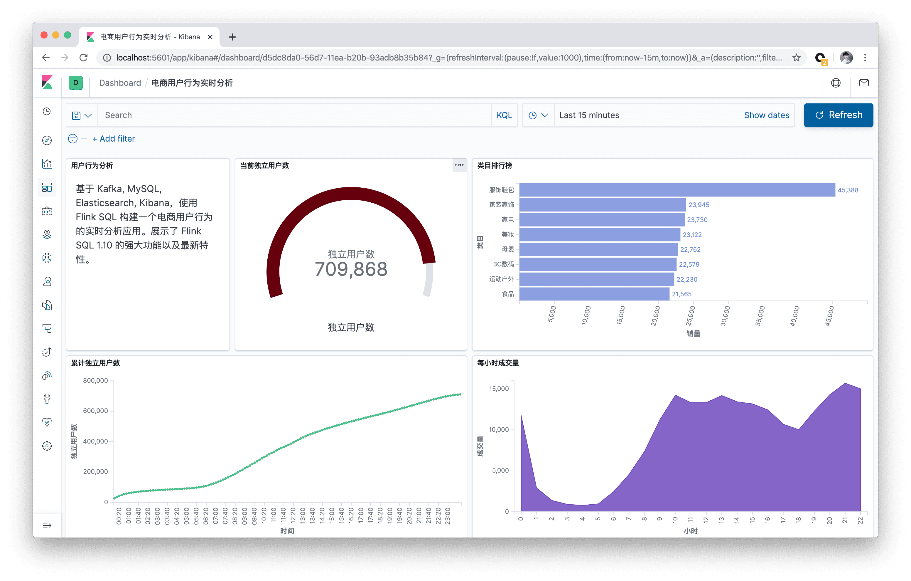
This article will use Flink SQL to build a real-time analytics application for e-commerce user behavior based on Kafka, MySQL, Elasticsearch, Kibana.

All the walkthroughs in this article will be executed on Flink SQL CLI, involving only SQL plain text, without a single line of Java/Scala code and no IDE installation.

The final result of this walkthrough.

Preparation

A Linux or MacOS computer with Docker and Java8.

Starting a container with Docker Compose

The components that this live demo relies on are all scheduled into containers, so they can be started with a single click via docker-compose. You can download the docker-compose.yml file automatically with the wget command, or you can download it manually.

1
2

mkdir flink-demo; cd flink-demo;
wget https://raw.githubusercontent.com/wuchong/flink-sql-demo/master/docker-compose.yml

The containers included in this Docker Compose are.

DataGen: Data generator. When the container starts, it automatically starts generating user behavior data and sends it to the Kafka cluster. The default is to generate 1000 data per second for about 3 hours. You can also change the speedup parameter of datagen in docker-compose.yml to adjust the generation rate (restart docker compose to take effect).
MySQL: integrated with MySQL 5.7, and a pre-created category table, pre-filled with mapping relationships between sub-categories and top-level categories, for subsequent use as a dimension table.
Kafka: Used primarily as a data source, the DataGen component automatically pours data into this container.
Zookeeper: Kafka container dependency.
Elasticsearch: Mainly stores the data produced by Flink SQL.
Kibana: visualizes the data in Elasticsearch.

Before starting the containers, it is recommended to modify the Docker configuration to adjust the resources to 4GB and 4 cores. To start all containers, just run the following command in the directory where docker-compose.yml is located.

`1`	`docker-compose up -d`

This command will automatically start all containers defined in the Docker Compose configuration in detached mode. You can use docker ps to see if the above five containers are started properly. You can also visit http://localhost:5601/ to see if Kibana is running properly.

Alternatively, all containers can be stopped with the following command.

`1`	`docker-compose down`

Download and install Flink Local Cluster

We recommend that users download and install Flink manually instead of starting Flink automatically via Docker. This is because it is more intuitive to understand the components, dependencies, and scripts of Flink.

Download the Flink 1.10.0 installation package and unzip it (unzip directory flink-1.10.0): https://www.apache.org/dist/flink/flink-1.10.0/flink-1.10.0-bin-scala_2.11.tgz
Go to the flink-1.10.0 directory: cd flink-1.10.0

Download the dependent jar packages and copy them to the lib/ directory with the following command, or you can download and copy them manually. Because we need to depend on each connector implementation when we run it.

wget -P ./lib/ https://repo1.maven.org/maven2/org/apache/flink/flink-json/1.10.0/flink-json-1.10.0.jar | \
    wget -P ./lib/ https://repo1.maven.org/maven2/org/apache/flink/flink-sql-connector-kafka_2.11/1.10.0/flink-sql-connector-kafka_2.11-1.10.0.jar | \
    wget -P ./lib/ https://repo1.maven.org/maven2/org/apache/flink/flink-sql-connector-elasticsearch6_2.11/1.10.0/flink-sql-connector-elasticsearch6_2.11-1.10.0.jar | \
    wget -P ./lib/ https://repo1.maven.org/maven2/org/apache/flink/flink-jdbc_2.11/1.10.0/flink-jdbc_2.11-1.10.0.jar | \
    wget -P ./lib/ https://repo1.maven.org/maven2/mysql/mysql-connector-java/5.1.48/mysql-connector-java-5.1.48.jar

Change taskmanager.numberOfTaskSlots in conf/flink-conf.yaml to 10, since we will be running multiple tasks at the same time.
Execute . /bin/start-cluster.sh to start the cluster. If it runs successfully, you can access Flink Web UI at http://localhost:8081. And you can see the number of available Slots is 10.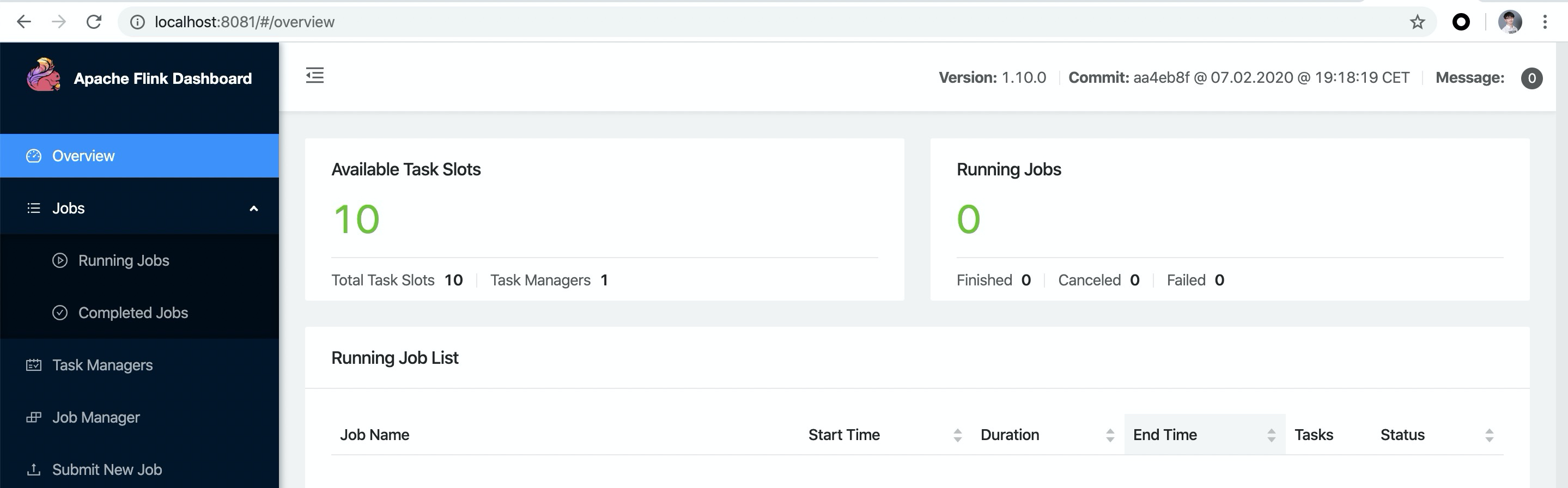
Execute bin/sql-client.sh embedded to start SQL CLI. You will see the following squirrel welcome screen.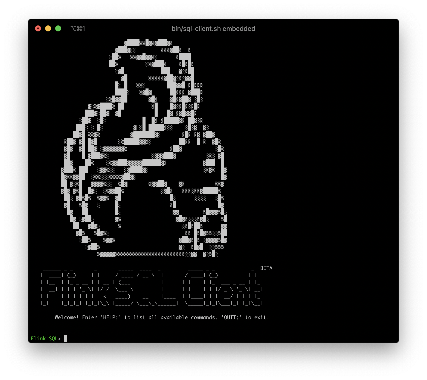

Creating Kafka Tables with DDL

The Datagen container continuously writes data to the user_behavior topic of Kafka after it is started. The data contains user behaviors (behaviors include click, buy, add, like) for one day on November 27, 2017, with each row representing one user behavior in JSON format consisting of user ID, product ID, product category ID, behavior type and time. The original dataset comes from the AliCloud Tianchi public dataset, and we would like to acknowledge it.

We can run the following command in the directory where docker-compose.yml is located to see the first 10 data generated in the Kafka cluster.

`1`	`docker-compose exec kafka bash -c 'kafka-console-consumer.sh --topic user_behavior --bootstrap-server kafka:9094 --from-beginning --max-messages 10'`

1
2
3

{"user_id": "952483", "item_id":"310884", "category_id": "4580532", "behavior": "pv", "ts": "2017-11-27T00:00:00Z"}
{"user_id": "794777", "item_id":"5119439", "category_id": "982926", "behavior": "pv", "ts": "2017-11-27T00:00:00Z"}
...

Once we have the data source, we can use the DDL to create and connect to this topic in Kafka. Execute the DDL in the Flink SQL CLI.

CREATE TABLE user_behavior (
    user_id BIGINT,
    item_id BIGINT,
    category_id BIGINT,
    behavior STRING,
    ts TIMESTAMP(3),
    proctime as PROCTIME(),   -- 通过计算列产生一个处理时间列
    WATERMARK FOR ts as ts - INTERVAL '5' SECOND  -- 在ts上定义watermark，ts成为事件时间列
) WITH (
    'connector.type' = 'kafka',  -- 使用 kafka connector
    'connector.version' = 'universal',  -- kafka 版本，universal 支持 0.11 以上的版本
    'connector.topic' = 'user_behavior',  -- kafka topic
    'connector.startup-mode' = 'earliest-offset',  -- 从起始 offset 开始读取
    'connector.properties.zookeeper.connect' = 'localhost:2181',  -- zookeeper 地址
    'connector.properties.bootstrap.servers' = 'localhost:9092',  -- kafka broker 地址
    'format.type' = 'json'  -- 数据源格式为 json
);

In addition to the 5 fields declared above in the format of the data, we also declare a virtual column that generates the processing time via the computed column syntax and the PROCTIME() built-in function. We also declare a watermark policy (tolerating 5 seconds of chaos) on the ts field via the WATERMARK syntax, and the ts field thus becomes an event time column. You can read the official documentation for more information about the time attribute and the DDL syntax

After successfully creating a Kafka table in the SQL CLI, you can view the currently registered tables and the table details by using show tables; and describe user_behavior;. We can also run SELECT * FROM user_behavior; directly in the SQL CLI to preview the data (press q to exit).

Next, we will go deeper into Flink SQL with three real-world scenarios.

Statistics of hourly volume

Creating Elasticsearch Tables with DDL

We first create an ES result table in the SQL CLI, which needs to save two main data according to the scenario requirements: hours, volume.

CREATE TABLE buy_cnt_per_hour ( 
    hour_of_day BIGINT,
    buy_cnt BIGINT
) WITH (
    'connector.type' = 'elasticsearch', -- 使用 elasticsearch connector
    'connector.version' = '6',  -- elasticsearch 版本，6 能支持 es 6+ 以及 7+ 的版本
    'connector.hosts' = 'http://localhost:9200',  -- elasticsearch 地址
    'connector.index' = 'buy_cnt_per_hour',  -- elasticsearch 索引名，相当于数据库的表名
    'connector.document-type' = 'user_behavior', -- elasticsearch 的 type，相当于数据库的库名
    'connector.bulk-flush.max-actions' = '1',  -- 每条数据都刷新
    'format.type' = 'json',  -- 输出数据格式 json
    'update-mode' = 'append'
);

We don’t need to create the buy_cnt_per_hour index in Elasticsearch beforehand, Flink Job will create it automatically.

Submit Query

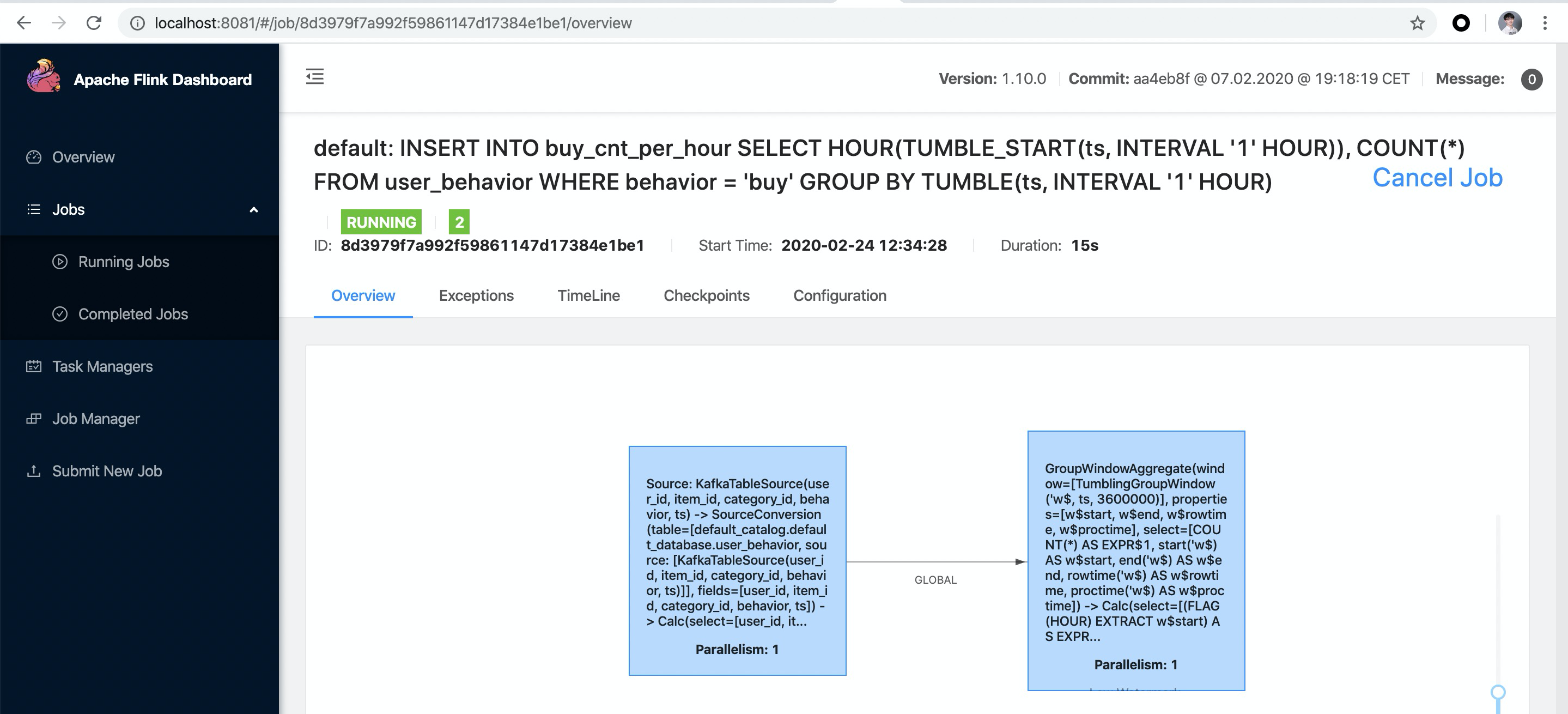
The hourly volume is the total number of “buys” made by users per hour. Therefore, we need to use the TUMBLE window function, which cuts the window by hour. Then each window will count the number of “buys” separately, which can be achieved by filtering out the “buys” first and then COUNT(*).

INSERT INTO buy_cnt_per_hour
SELECT HOUR(TUMBLE_START(ts, INTERVAL '1' HOUR)), COUNT(*)
FROM user_behavior
WHERE behavior = 'buy'
GROUP BY TUMBLE(ts, INTERVAL '1' HOUR);

Here we use the HOUR built-in function to extract the value of the first hour of the day from a TIMESTAMP column. INSERT INTO is used to continuously insert the results of query into the es results table defined above (think of the es results table as a materialized view of query). Also read this document to learn more about window aggregation: https://ci.apache.org/projects/flink/flink-docs-release-1.10/dev/table/sql/queries.html#group-windows

After running the above query in Flink SQL CLI, you can see the submitted task in Flink Web UI, which is a streaming task and thus will keep running.

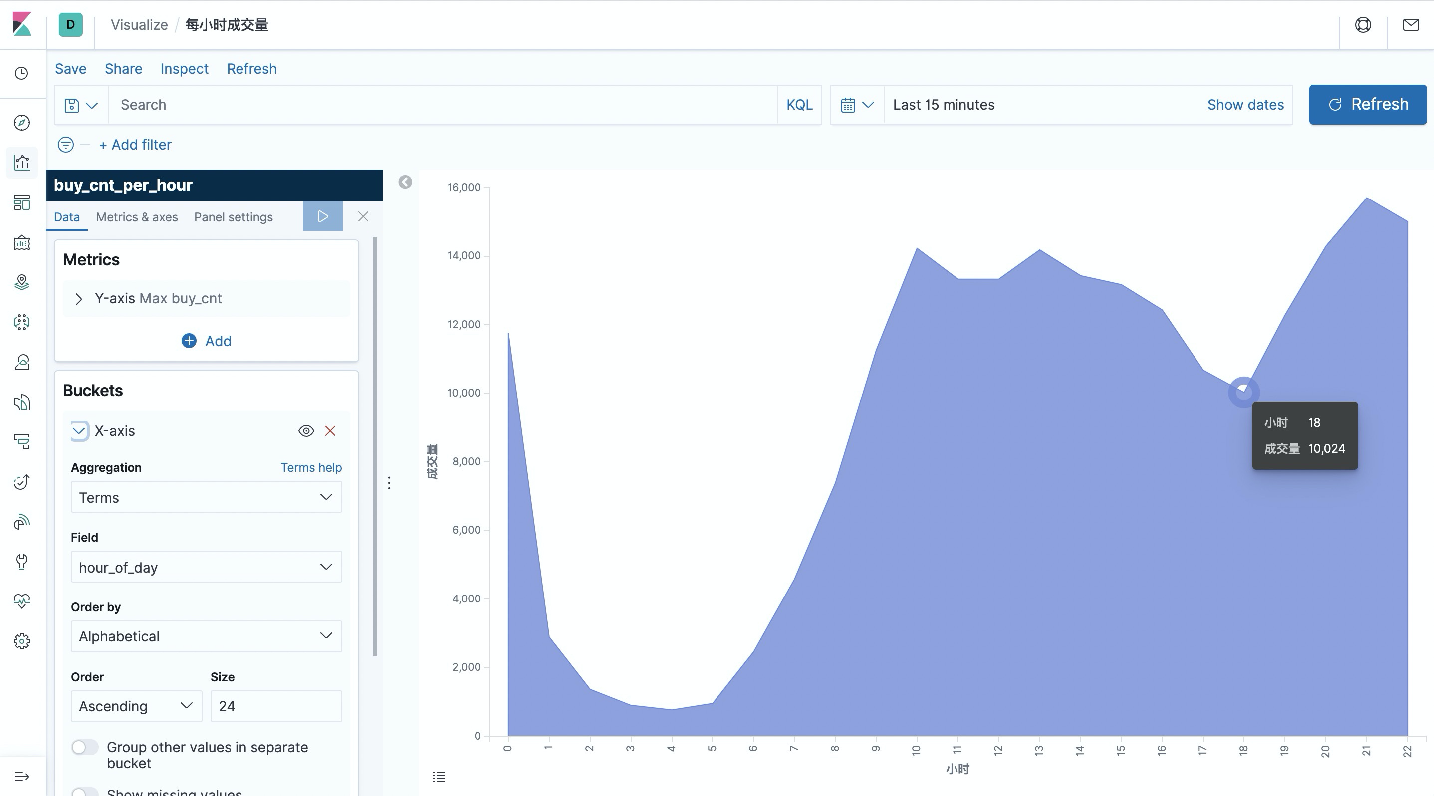
You can see that the early morning hours are the low point of the day in terms of volume.

Visualize results with Kibana

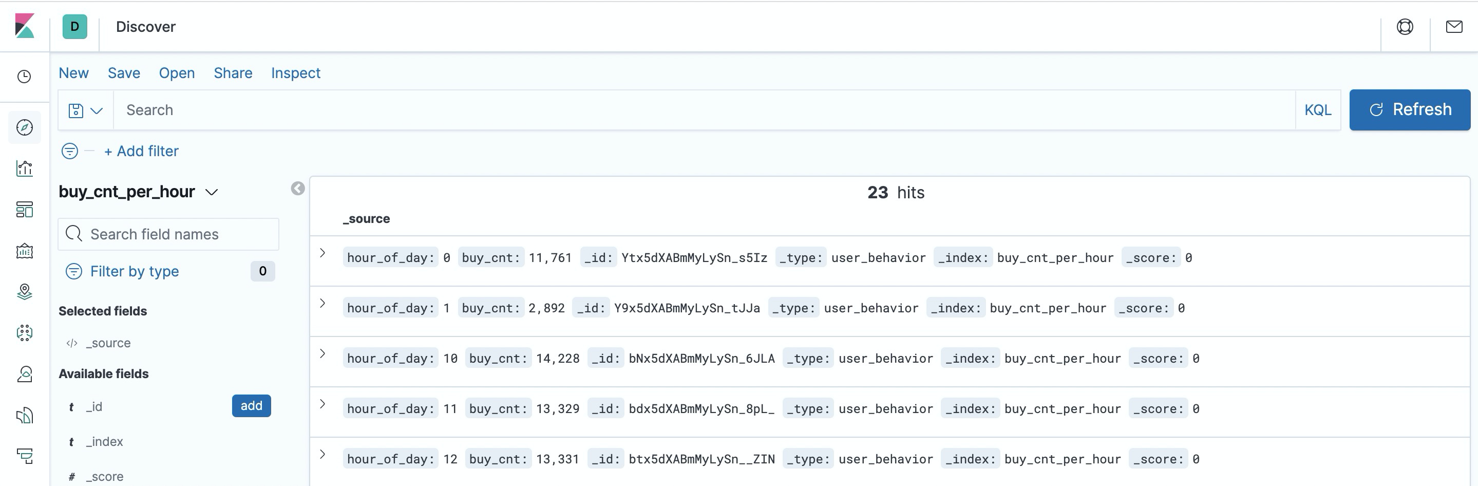
We have started the Kibana container via Docker Compose and can access Kibana via http://localhost:5601. First we need to configure an index pattern first. Click Management in the left toolbar and you will find Index Patterns. Click Create Index Pattern and then create index pattern by entering the full index name buy_cnt_per_hour. Once created, Kibana will know our indexes and we can start exploring the data.

First click the “Discovery” button on the left toolbar, and Kibana will list the contents of the index you just created.

Next, let’s create a Dashboard to display each visualization view. Click “Dashboard” on the left side of the page to create a Dashboard called “User Behavior Log Analysis”. Then click “Create New” to create a new view, select “Area” area map, choose “buy_cnt_per_hour " index and draw the volume area map as configured in the screenshot below (left side) and save it as “Volume per hour”.

Count the cumulative number of unique users per 10 minutes a day

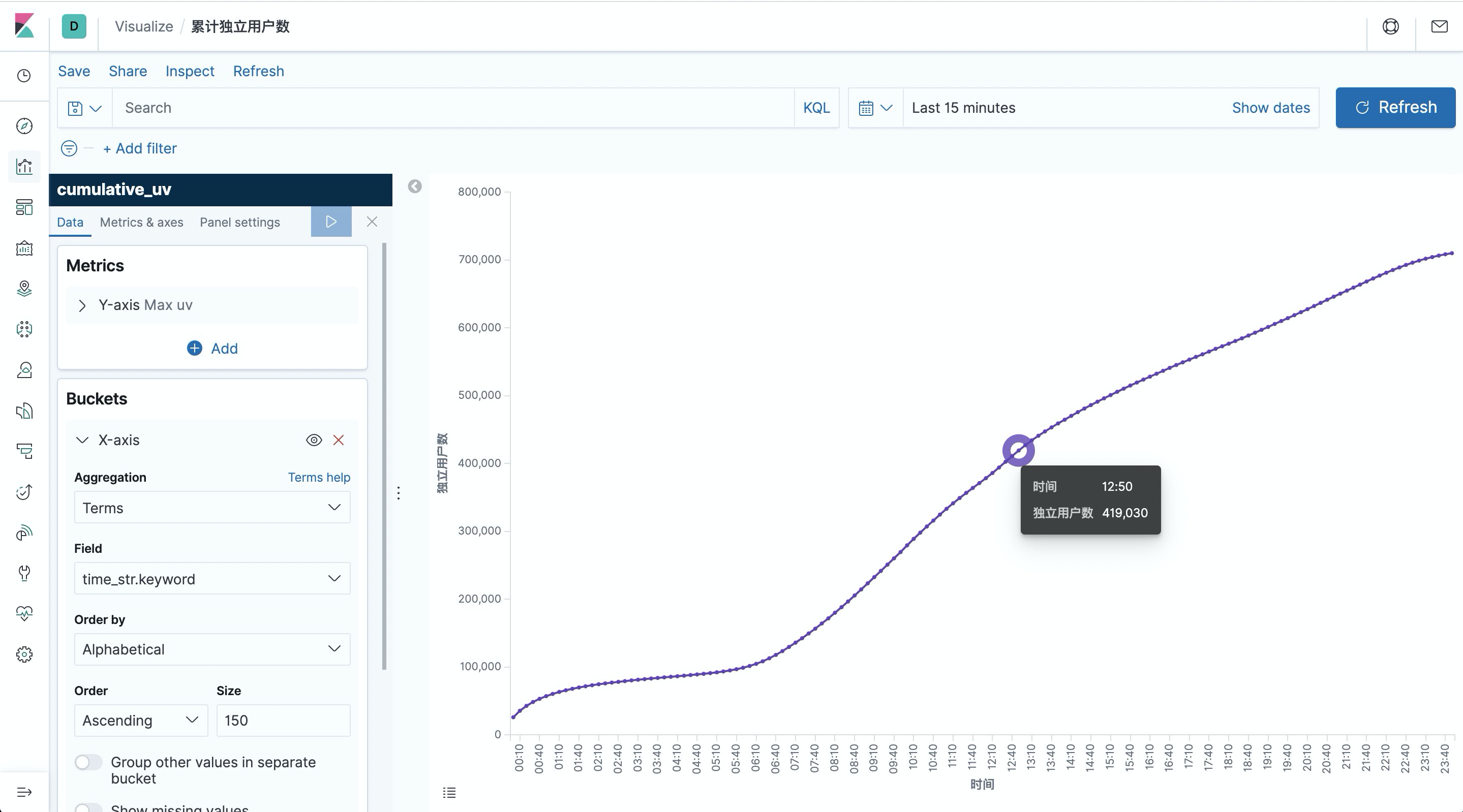
Another interesting visualization is to count the cumulative number of unique users (uv) at each moment of the day, i.e., the uv count at each moment represents the total uv count from point 0 to the current moment, so the curve must be monotonically increasing.

We still start by creating an Elasticsearch table in the SQL CLI to store the result summary data. There are two main fields: time and cumulative uv count.

CREATE TABLE cumulative_uv (
    time_str STRING,
    uv BIGINT
) WITH (
    'connector.type' = 'elasticsearch',
    'connector.version' = '6',
    'connector.hosts' = 'http://localhost:9200',
    'connector.index' = 'cumulative_uv',
    'connector.document-type' = 'user_behavior',
    'format.type' = 'json',
    'update-mode' = 'upsert'
);

To achieve this curve, we can first calculate the current minute of each data by OVER WINDOW, and the current cumulative uv (the number of unique users from point 0 to the current row). The uv count is done with the built-in COUNT(DISTINCT user_id), and Flink SQL has a lot of internal optimizations for COUNT DISTINCT, so you can use it without worry.

CREATE VIEW uv_per_10min AS
SELECT 
  MAX(SUBSTR(DATE_FORMAT(ts, 'HH:mm'),1,4) || '0') OVER w AS time_str, 
  COUNT(DISTINCT user_id) OVER w AS uv
FROM user_behavior
WINDOW w AS (ORDER BY proctime ROWS BETWEEN UNBOUNDED PRECEDING AND CURRENT ROW);

Here we use SUBSTR and DATE_FORMAT and || built-in functions to convert a TIMESTAMP field into a time string in 10 minutes, e.g.: 12:10, 12:20. More about OVER WINDOW can be found in the documentation: https://ci.apache.org/projects/flink/flink-docs-release-1.10/dev/table/sql/queries.html#aggregations

We also use the CREATE VIEW syntax to register a query as a logical view that can be easily referenced in subsequent queries, which facilitates the disassembly of complex queries. Note that creating a logical view does not trigger job execution and the results of the view do not land, so it is very lightweight to use and has no additional overhead. Since uv_per_10min produces one output for each input data, it is more stressful for storage. We can do another aggregation based on uv_per_10min based on the time in minutes, so that only one point per 10 minutes will be stored in Elasticsearch, which will be much less stressful for Elasticsearch and Kibana visual rendering.

INSERT INTO cumulative_uv
SELECT time_str, MAX(uv)
FROM uv_per_10min
GROUP BY time_str;

After submitting the above query, create an index pattern for cumulative_uv in Kibana, then create a Line line chart in Dashboard, select cumulative_uv index, draw the cumulative number of unique users curve according to the configuration in the screenshot below (left side) and save it.

The last interesting visualization is the category ranking, so as to understand which categories are the pillar categories. However, since the category classification in the source data is too fine (about 5000 categories) to be meaningful for the leaderboard, we would like to approximate it to the top categories. So I pre-prepared the mapping data between sub-categories and top categories in the mysql container to be used as a dimension table.

The MySQL table is created in the SQL CLI and later used as a dimension table query.

CREATE TABLE category_dim (
    sub_category_id BIGINT,  -- 子类目
    parent_category_id BIGINT -- 顶级类目
) WITH (
    'connector.type' = 'jdbc',
    'connector.url' = 'jdbc:mysql://localhost:3306/flink',
    'connector.table' = 'category',
    'connector.driver' = 'com.mysql.jdbc.Driver',
    'connector.username' = 'root',
    'connector.password' = '123456',
    'connector.lookup.cache.max-rows' = '5000',
    'connector.lookup.cache.ttl' = '10min'
);

We also create an Elasticsearch table to store the category statistics.

CREATE TABLE top_category (
    category_name STRING,  -- 类目名称
    buy_cnt BIGINT  -- 销量
) WITH (
    'connector.type' = 'elasticsearch',
    'connector.version' = '6',
    'connector.hosts' = 'http://localhost:9200',
    'connector.index' = 'top_category',
    'connector.document-type' = 'user_behavior',
    'format.type' = 'json',
    'update-mode' = 'upsert'
);

In the first step we complete the class names through dimensional table association. We still use CREATE VIEW to register the query as a view and simplify the logic. The dimensional table association uses the temporal join syntax, see the documentation for more information: https://ci.apache.org/projects/flink/flink-docs-release-1.10/dev/table/streaming/joins.html#join-with-a-temporal-table

CREATE VIEW rich_user_behavior AS
SELECT U.user_id, U.item_id, U.behavior, 
  CASE C.parent_category_id
    WHEN 1 THEN '服饰鞋包'
    WHEN 2 THEN '家装家饰'
    WHEN 3 THEN '家电'
    WHEN 4 THEN '美妆'
    WHEN 5 THEN '母婴'
    WHEN 6 THEN '3C数码'
    WHEN 7 THEN '运动户外'
    WHEN 8 THEN '食品'
    ELSE '其他'
  END AS category_name
FROM user_behavior AS U LEFT JOIN category_dim FOR SYSTEM_TIME AS OF U.proctime AS C
ON U.category_id = C.sub_category_id;

Finally, the number of events for buy is counted and written to Elasticsearch, grouped by category name.

INSERT INTO top_category
SELECT category_name, COUNT(*) buy_cnt
FROM rich_user_behavior
WHERE behavior = 'buy'
GROUP BY category_name;

After submitting the above query, create an index pattern for top_category in Kibana, then create a Horizontal Bar bar in Dashboard, select the top_category index, draw the category ranking according to the configuration in the screenshot below (left side), and save it.

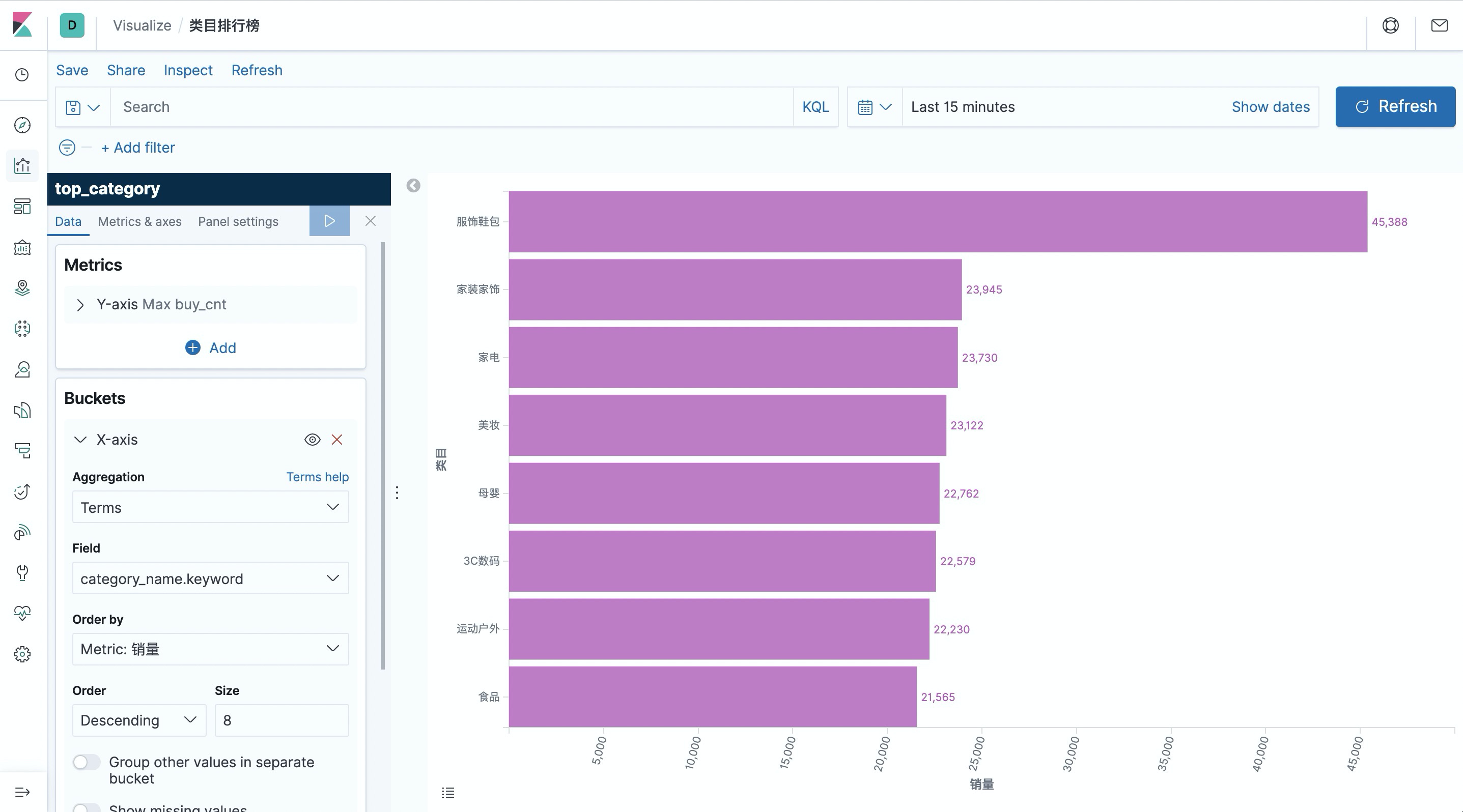
As you can see, the volume of “服饰鞋包” is far ahead of other categories.

Kibana also provides very rich graphing and visualization options, interested users can use Flink SQL to analyze the data in more dimensions, and use Kibana to display the visualization graph and observe the real-time changes of the graph data.

Ending

In this article, we show how to use Flink SQL to integrate Kafka, MySQL, Elasticsearch and Kibana to quickly build a real-time analytics application. The whole process can be done without a single line of Java/Scala code, using SQL plain text. We hope this article will give readers an idea of the ease of use and power of Flink SQL, including easy connection to various external systems, native support for event time and chaotic data processing, dimensional table association, rich built-in functions, and more.

Reference http://wuchong.me/blog/2020/02/25/demo-building-real-time-application-with-flink-sql/

Table of Contents