The company’s Jupyter environment supports PySpark. this makes it very easy to use PySpark to connect to Hive queries and use. Since I had no prior exposure to Spark at all, I put together some reference material.
Spark Context
The core module in PySpark is SparkContext (sc for short), and the most important data carrier is RDD, which is like a NumPy array or a Pandas Series, and can be regarded as an ordered set of items. The RDD is like a NumPy array or a Pandas Series, which can be regarded as an ordered collection of items, but these items do not exist in the memory of the driver, but are divided into many partitions, and the data of each partition exists in the memory of the cluster executor.
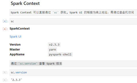
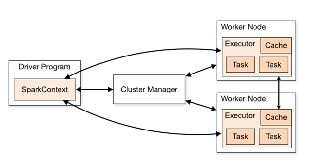
SparkContext is the main entry point of Spark, if you consider Spark cluster as server, Spark Driver is the client, SparkContext is the core of the client; as the comment says SparkContext is used to connect to Spark cluster, create RDD, accumlator, broadcast variables, which is equivalent to the main function of the application.
Only one active SparkContext can exist in each JVM, and you must call stop() to close the previous SparkContext before creating a new one.
Spark Session
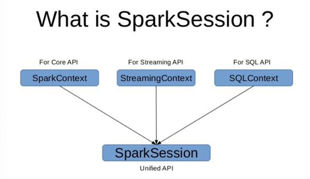
Before Spark 2.0, SparkContext was the structure for all Spark functions, and the driver connected to the cluster (via resource manager) through SparkContext, because before 2.0, RDD was the foundation of Spark. If you need to create a SparkContext, you need SparkConf to configure the content of SparkContext through Conf.
After Spark2.0, Spark Session is also an entry point for Spark, in order to introduce dataframe and dataset APIs, while retaining the functionality of the original SparkContext, if you want to use the HIVE, SQL, Streaming APIs, you need Spark Session is the entry point.
SparkSession not only provides access to all the spark functions that sparkContext has, but also provides APIs for handling DataFrame and DataSet.
Here’s how to create a SparkSession.
The following are the parameters of SparkContext.
- master - It is the URL of the cluster to connect to.
- appName - The name of your job.
- sparkHome - The Spark installation directory.
- pyFiles - The .zip or .py files to send to the cluster and add to the PYTHONPATH.
- environment - Work node environment variable.
- batchSize - The number of Python objects represented as a single Java object. Set 1 to disable batching, 0 to automatically select batch size based on object size, or -1 to use unlimited batch size.
- serializer - The RDD serializer.
- Conf - An object of L {SparkConf} to set all Spark properties.
- gateway - Use the existing gateway and JVM, otherwise initialize the new JVM.
- JSC - JavaSparkContext instance.
- profiler_cls - A custom class of Profiler used for performance analysis (default is profiler.BasicProfiler).
In the above parameters, master and appname are mainly used.
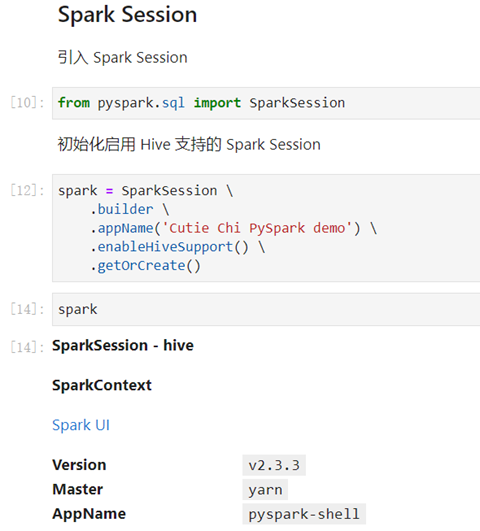
Here’s how we can create a SparkSession using Hive support.
RDD, Dataset and DataFrame
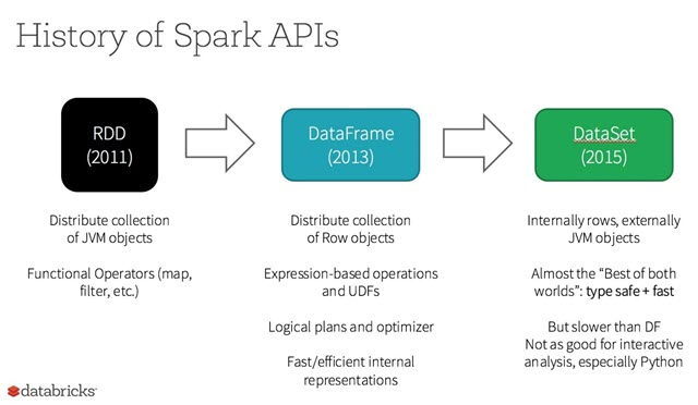
RDD
An RDD is an immutable collection of distributed elements of your data, distributed across nodes in a cluster, that can be processed in parallel by several underlying APIs that provide transformation and processing.
Scenarios for using RDDs:
- You want to be able to perform the most basic transformations, processing and control of your data set.
- Your data is unstructured, such as streaming media or character streams.
- You want to process your data through functional programming rather than domain-specific representations.
- you don’t want to define a schema as in columnar processing, processing or accessing data attributes by name or field.
- you do not care for some of the optimization and performance benefits that can be gained by structured and semi-structured data processing through DataFrame and Dataset.
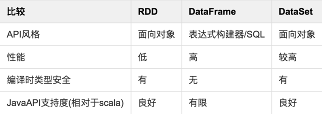
Pros.
- Powerful, with many built-in function operations, group, map, filter, etc., to facilitate the handling of structured or unstructured data
- object-oriented programming, direct storage of java objects, type conversion is also safe
Disadvantages.
- because it is basically the same as hadoop universal, so there is no optimization for special scenarios, such as for structured data processing compared to sql to very troublesome
- the default is the java serial number method, serialization results are relatively large, and the data is stored in the java heap memory, resulting in more frequent gc
DataFrame
DataFrame is a distributed data set based on RDD, similar to the two-dimensional tables in traditional databases. dataFrame introduces schema.
RDD and DataFrame comparison.
- Similarities: Both are immutable distributed elastic datasets.
- Differences: DataFrame datasets are stored by specified columns, i.e. structured data. Similar to a table in a traditional database.
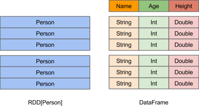
The above figure visualizes the difference between DataFrame and RDD.
- The RDD [Person] on the left has Person as the type parameter, but the Spark framework itself does not know the internal structure of the Person class. The DataFrame on the right side, however, provides detailed structure information, so that Spark SQL can clearly know which columns are contained in the dataset and what the name and type of each column are. dataFrame has more information about the structure of the data, i.e. schema.
- RDD is a distributed collection of Java objects. dataFrame is a distributed collection of Row objects.
- DataFrame provides richer arithmetic than RDD, but the more important feature is to improve the execution efficiency, reduce data reading and the optimization of execution plan, such as filter push down, crop, etc.
Advantages.
- Structured data processing is very convenient, supporting kv data such as Avro, CSV, elastic search, and Cassandra, as well as traditional data tables such as HIVE tables, MySQL, etc.
- targeted optimization, because the data structure meta information spark has been saved, serialization does not need to bring meta information, greatly reducing the size of serialization, and the data is saved in off-heap memory, reducing the number of gc.
- hive compatible, support hql, udf, etc.
Disadvantages.
- No type conversion safety check at compile time, runtime to determine if there is a problem
- for object support is not friendly, rdd internal data stored directly in java objects, dataframe memory storage is row objects and can not be custom objects
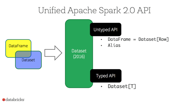
DataSet
A Dataset is a strongly typed domain-specific object that can be transformed in parallel by functional or relational operations. Each Dataset has an untyped view called a DataFrame, which is a dataset of rows. This DataFrame is a Dataset of type Row, i.e. Dataset[Row].
You can think of a DataFrame as an alias for a collection of some generic object Dataset[Row], and a row is a generic untyped JVM object. In contrast, a Dataset is a collection of JVM objects with explicit type definitions, specified by the Case Class you define in Scala or the Class in Java.
Datasets are “lazy”, triggering computation only when an action is performed. Essentially, a dataset represents a logical plan that describes the computation required to produce the data. When an action is performed, Spark’s query optimizer optimizes the logical plan and generates an efficient parallel and distributed physical plan.
The main difference between a DataSet and an RDD is that a DataSet is a domain-specific collection of objects; however, an RDD is a collection of any objects. the DataSet API is always strongly typed; and it is possible to optimize using these patterns, however, an RDD is not.
Advantages.
- dataset integrates the advantages of rdd and dataframe, supporting both structured and unstructured data
- Same support for custom object storage as rdd
- Same as dataframe, supports sql queries for structured data
- Out-of-heap memory storage, gc friendly
- Type conversion safe, code friendly
- Officially recommended to use dataset
Spark DataFrame and Pandas DataFrame
Origin of DataFrame
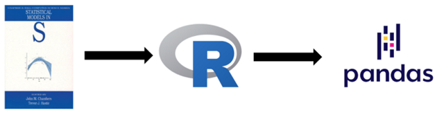
The earliest “DataFrame” (which began to be called “data frame”), originated from the S language developed by Bell Labs. data frame" was released in 1990, and its concepts are detailed in Chapter 3 of “Statistical Models of the S Language”, which highlights the matrix origin of the dataframe. The book describes DataFrame as looking very much like a matrix and supporting matrix-like operations; at the same time, it looks very much like a relational table.
The R language, an open source version of the S language, released its first stable version in 2000 and implemented dataframes. pandas was developed in 2009, and the concept of DataFrame was introduced in Python. These DataFrames are all homogeneous and share the same semantics and data model.
DataFrame Data Model
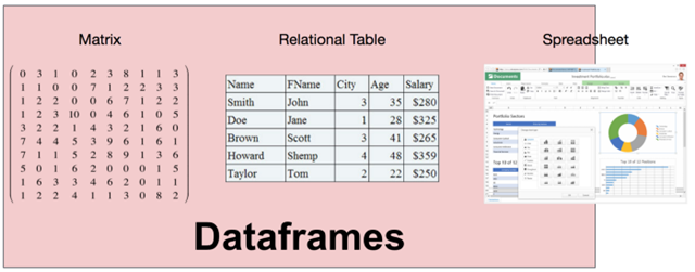
The need for a DataFrame comes from viewing data as a matrix and a table. However, matrices contain only one data type, which is too restrictive, and relational tables require that the data must first have a schema defined; for a DataFrame, its column types can be inferred at runtime and do not need to be known in advance, nor are all columns required to be of one type. Thus, a DataFrame can be thought of as a combination of a relational system, a matrix, or even a spreadsheet program (typically Excel).
Compared to relational systems, DataFrames have several particularly interesting properties that make DataFrames unique.
Guaranteed order, column and row symmetry
First, DataFrames are ordered in both row and column directions; and rows and columns are first-class citizens and are not treated differently.
Take pandas for example, when a DataFrame is created, the data is ordered in both rows and columns; therefore, you can use position to select data in both rows and columns.
|
|
Those familiar with numpy (the numerical computation library containing definitions of multidimensional arrays and matrices) can see that this feature is very familiar, and thus the matrix nature of DataFrame can be seen.
Rich API
The DataFrame API is very rich, spanning relational (e.g. filter, join), linear algebra (e.g. transpose, dot) and spreadsheet-like (e.g. pivot) operations.
Again using pandas as an example, a DataFrame can do transpose operations to get rows and columns to line up.
Intuitive syntax for interactive analysis
Users can continuously explore DataFrame data, query results can be reused by subsequent results, and very complex operations can be very easily combined programmatically, making it well suited for interactive analysis.
Heterogeneous data allowed in columns
The DataFrame type system allows for the presence of heterogeneous data in a column, for example, an int column allows for the presence of string type data, which may be dirty data. This makes DataFrame very flexible.
Data Model
We can now formally define what a DataFrame really is.
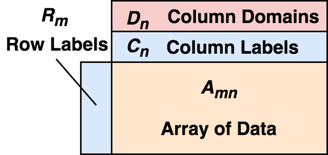
A DataFrame consists of a two-dimensional array of mixed types, row labels, column labels, and types (types or domains). On each column, the type is optional and can be inferred at runtime. In terms of rows, a DataFrame can be viewed as a mapping of row labels to rows, with guaranteed order between rows; in terms of columns, it can be viewed as a mapping of column types to column labels to columns, again with guaranteed order between columns.
The existence of row labels and column labels makes it very convenient to select data.
|
|
Here index and columns are the row and column labels respectively. We can easily select a period of time (row selection) and several columns (column selection) of data. Of course, this is based on the fact that the data is stored sequentially.
This sequential storage makes DataFrame very suitable for statistical work.
|
|
As we can see from the example, just because the data is stored in order, we can keep the index unchanged and move down one row as a whole, so that yesterday’s data goes to today’s row, and then when we take the original data and subtract the displaced data, because DataFrame will automatically do alignment by label, so for a date, it is equivalent to subtracting the previous day’s data from the day’s data, so that we can do something like ring-by-ring operation. This is incredibly convenient. I’m afraid that for a relational system, you’d need to find a column to use as a join condition, and then do the subtraction, etc. Finally, for empty data, we can also fill in the previous row (ffill) or the next row (bfill). Trying to achieve the same effect in a relational system would require a lot of work.
Spark’s DataFrame
Spark brings the concept of “DataFrame” to the Big Data space. Spark DataFrame only contains the semantics of relational tables, the schema needs to be determined, and the data is not guaranteed to be sequential.
Difference between Pandas DataFrame and Spark DataFrame
TODO
DataFrameReader class and DataFrameWriter class
DataFrameReader class
Reading data from an external storage system and returning a DataFrame object is usually accessed using SparkSession.read. The common syntax is to first call the format() function to specify the format of the input data, and then call the load() function to load the data from the data source and return the DataFrame object.
|
|
For the different formats, the DataFrameReader class has subdivided functions to load the data.
|
|
DataFrame can also be constructed from JDBC URLs via jdbc
|
|
DataFrameWriter class
Used to write a DataFrame to an external storage system, accessible via DataFrame.write.
Function Comments.
- format(source): Specify the format of the source of the underlying output
- mode(saveMode): Specify the behavior of the data storage when the data or table already exists. Save modes are: append, overwrite, error, and ignore.
- saveAsTable(name, format=None, mode=None, partitionBy=None, **options): store the DataFrame as a table
- save(path=None, format=None, mode=None, partitionBy=None, **options): store the DataFrame to the data source
For different formats, the DataFrameWriter class has subdivision functions to load the data.
|
|
Storing the DataFrame content to the source.
|
|
To store the contents of a DataFrame into a table.
|
|
PySpark Interaction with Hive Database
|
|
Spark DataFrame operations
Spark dataframe is immutable, so each return is a new dataframe
Column operation
|
|
Conditional filtering of data
Select data
aggregate function
Consolidated Data Sheet