What can we learn from TiDB?

What is TiDB

TiDB is an open source distributed relational database designed and developed by PingCAP, which is a converged distributed database product that supports both Online Transaction Processing and Online Analytical Processing (HTAP).

Five core features

• One-click horizontal scaling or shrinking: On-demand online scaling or shrinking of compute and storage respectively, transparent to application operators and maintenance personnel during scaling or shrinking.

• Financial High Availability: Data replicas are synchronized with transaction logs via Multi-Raft protocol, and only commits when most transactions are written successfully, ensuring strong data consistency and not affecting data availability when a few replicas fail.

• Real-time HTAP: Provides row storage engine TiKV, column storage engine TiFlash stable/tiflash-overview), TiFlash replicates data from TiKV in real time via Multi-Raft Learner protocol to ensure strong data consistency between TiKV, the row storage engine, and TiFlash, the column storage engine.

• Cloud-native distributed database: enables tooling and automation of deployment in public, private, and hybrid clouds.

• Compatible with MySQL 5.7 protocol and MySQL ecosystem: applications can migrate from MySQL to TiDB with no or little code changes.

  Provide rich data migration tools to help applications complete data migration easily.

Architecture Analysis

In terms of kernel design, TiDB distributed database splits the overall architecture into several modules, and each module communicates with each other to form a complete TiDB system. The corresponding architecture diagram is as follows.

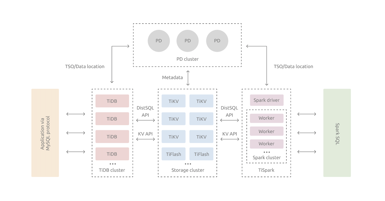
• TiDB Server: The SQL layer, exposing the connection endpoint of MySQL protocol, is responsible for accepting connections from clients, performing SQL parsing and optimization, and finally generating distributed execution plans. or TiFlash).
• PD (Placement Driver) Server: The meta information management module of the whole TiDB cluster, responsible for storing the real-time data distribution of each TiKV node and the overall topology of the cluster, providing TiDB Dashboard control interface, and assigning transaction IDs to distributed transactions.
• TiKV Server, the storage node, is responsible for storing data. Externally, TiKV is a distributed Key-Value storage engine that provides transactions. The basic unit for storing data is Region, each Region is responsible for storing data in a Key Range (left-closed right-open interval from StartKey to EndKey), and each TiKV node is responsible for multiple Regions.

SQL execution process

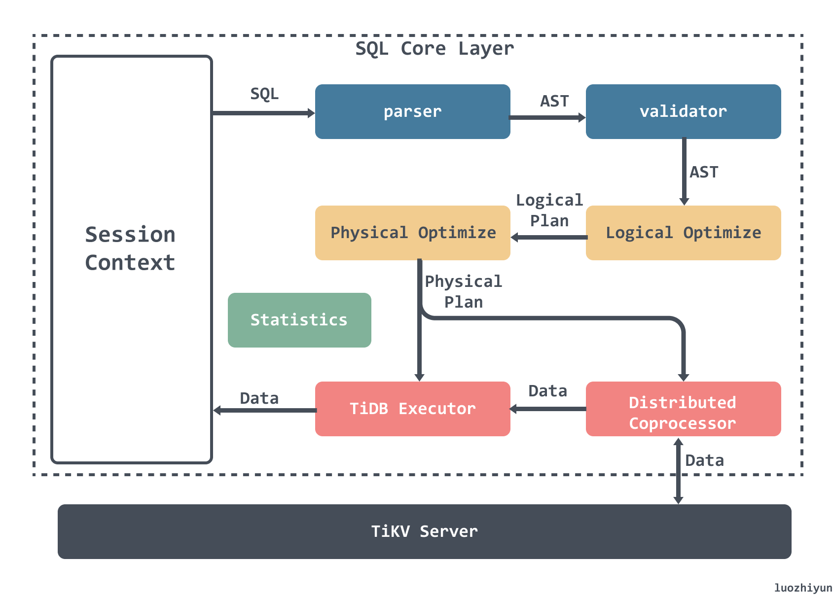
The whole SQL execution process consists of the following parts.

• Parser & validator: parsing the text into structured data, i.e. Abstract Syntax Tree (AST), and then validating the legitimacy of the AST.
• Logical Optimize: apply some optimization rules to the input logical execution plan in order to make the whole logical execution plan better. For example, associative subquery de-association, Max/Min elimination, predicate push-down, Join reordering, etc.
• Physical Optimize Physical Optimize: used to create a physical execution plan for the logical execution plan generated in the previous stage. The optimizer selects a specific physical implementation for each operator in the logical execution plan. There may be multiple physical implementations of the same logical operator, such as LogicalAggregate, which can be either HashAggregate using a hashing algorithm or StreamAggregate in a streaming format.
• Coprocessor: In TiDB, the computation is done in Region, the SQL layer will analyze the Key Range of the data to be processed, then divide these Key Ranges into several Key Ranges according to the Region information obtained from PD, and finally send these requests to the corresponding Region, and the module that computes the TiKV data corresponding to each Region is called Coprocessor.
• TiDB Executor: TiDB will merge and aggregate the data returned by Region for settlement.

Building AST syntax tree

For example, the following SQL statement.

1

select id,name,age from student where age>1 and name='pingcap';

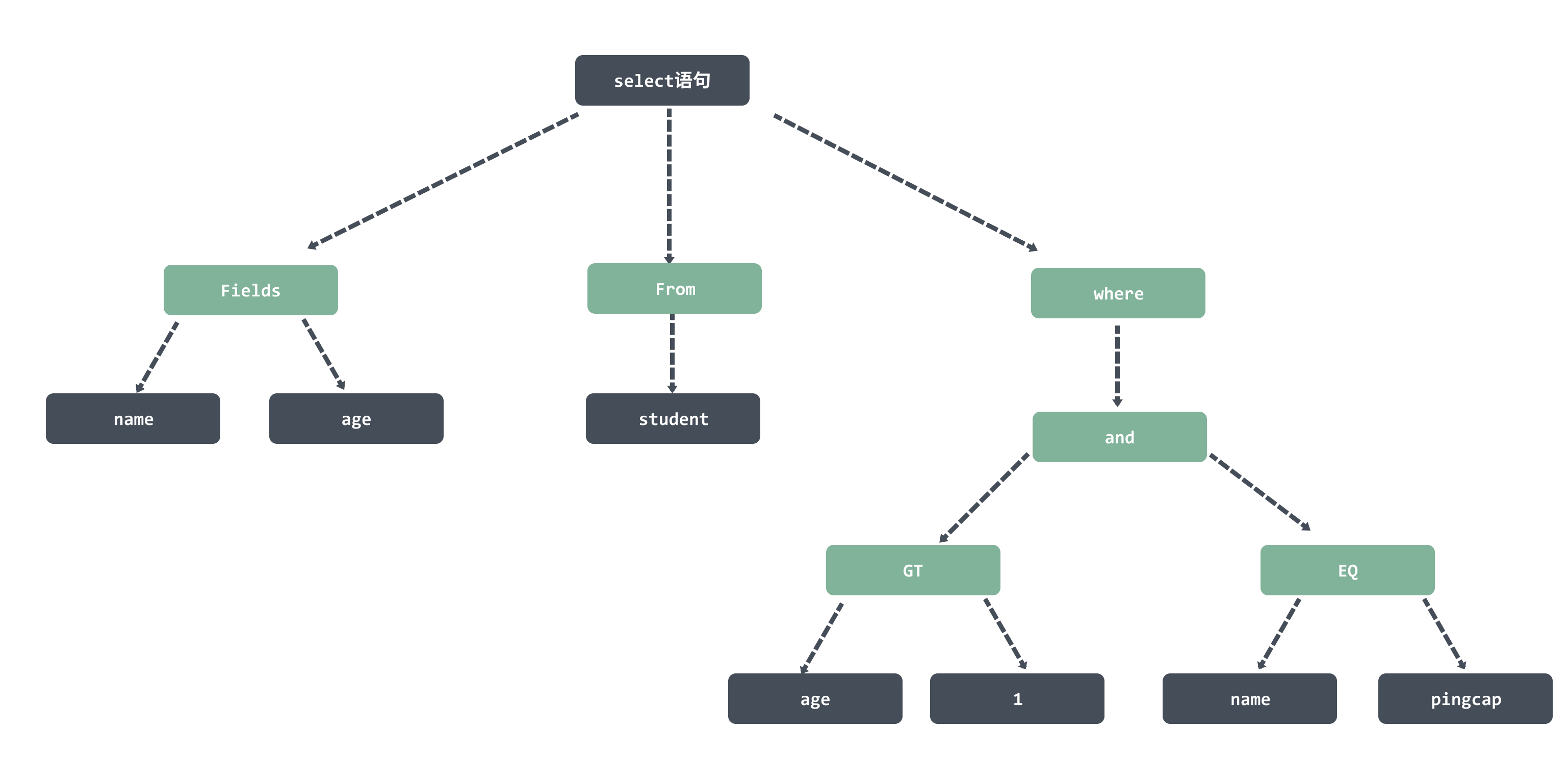
It is parsed to generate a syntax tree, which is then stored in the ast.StmtNode data structure.

 1
 2
 3
 4
 5
 6
 7
 8
 9
10
11

type SelectStmt struct {
    dmlNode 
    *SelectStmtOpts 
    Distinct bool 
    From *TableRefsClause 
    Where ExprNode 
    Fields *FieldList 
    GroupBy *GroupByClause 
    Having *HavingClause
    ...
}

Build the execution plan

Next, we will build the execution plan based on the node information of the ast syntax tree. Since the above SQL is relatively simple, let’s change to a function with aggregation to see the execution plan we generated.

1

select * from test1 where b=5 or ( b>5 and (b>6 or b <8)  and b<12) ;

Our execution plan will then be generated based on the ast syntax tree generated from this SQL.

The execution plan consists of the following operators.

• DataSource : this is the data source, that is, the table, that is, the student table above.
• LogicalSelection: This is the filter condition after where.
• Projection: this is the corresponding select followed by the field.

LogicalOptimization

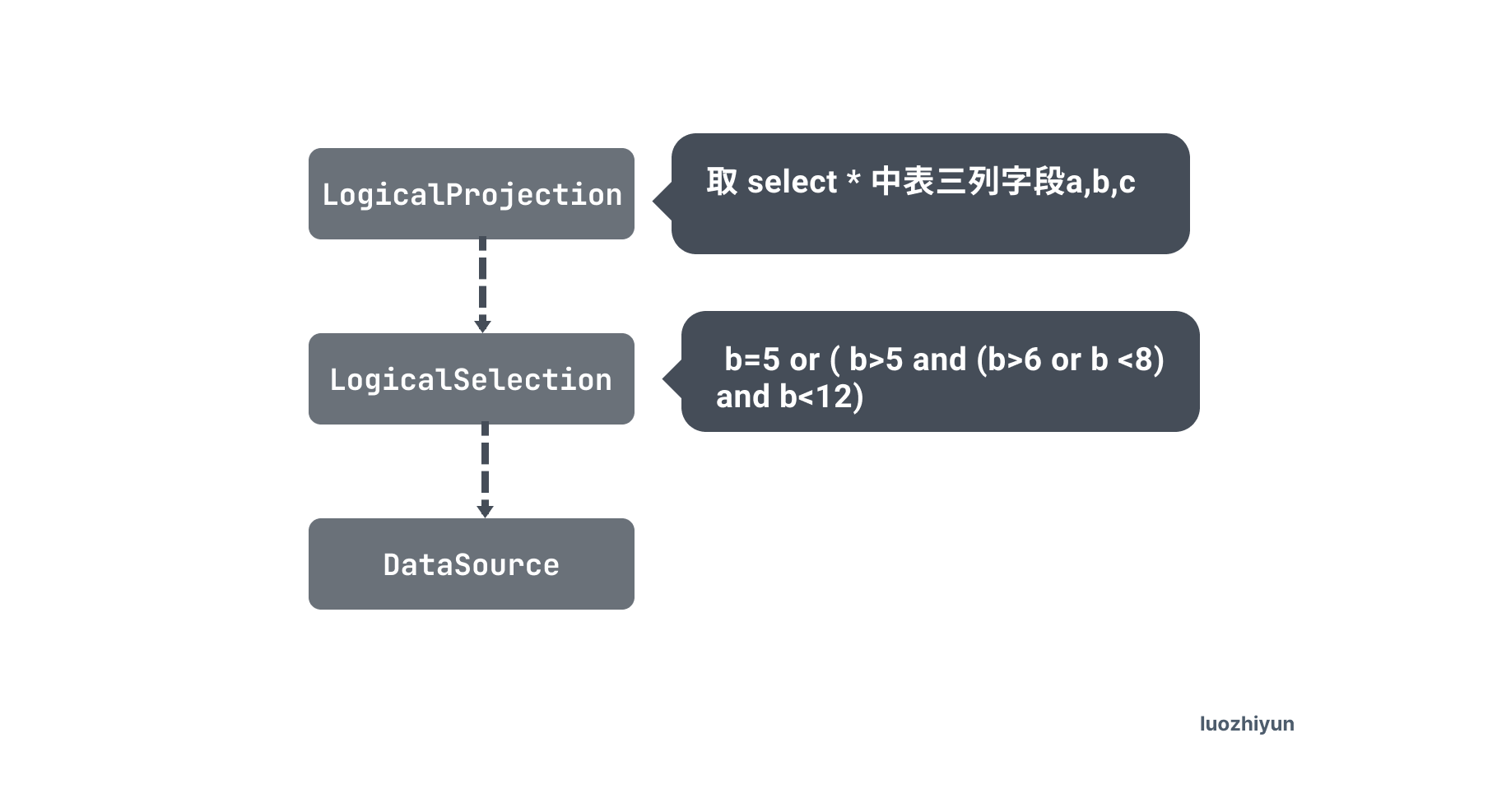
After the logicalOptimize logical optimization is executed, the execution plan becomes the following.

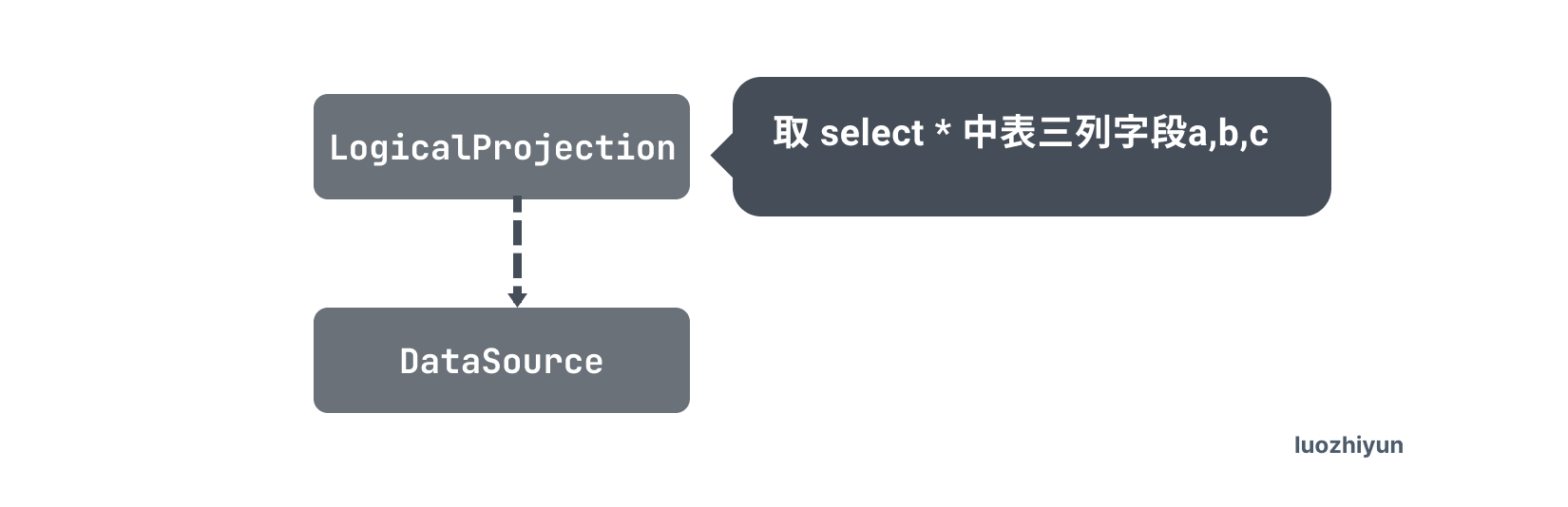
The Selection operator is pushed down into the DataSource operator, which is called Predicate Push Down (PDD) optimization. Predicate Push Down(PDD) optimization.

The basic idea of Predicate Push Down is to move the filter expression as close to the DataSource as possible so that irrelevant data can be skipped directly when it is actually executed.

The pushed-down filter operators are held in the pushedDownConds of the DataSource. pushedDownConds expands to a binary tree structure.

Because the index bottom is ordered, it is important to turn this tree into a scan interval.

In addition to predicate push-down optimization, TiDB already supports the following optimization rules.

 1
 2
 3
 4
 5
 6
 7
 8
 9
10
11
12
13
14
15
16

var optRuleList = []logicalOptRule{
    &gcSubstituter{},
    &columnPruner{},
    &buildKeySolver{},
    &decorrelateSolver{},
    &aggregationEliminator{},
    &projectionEliminator{},
    &maxMinEliminator{},
    &ppdSolver{},
    &outerJoinEliminator{},
    &partitionProcessor{},
    &aggregationPushDownSolver{},
    &pushDownTopNOptimizer{},
    &joinReOrderSolver{},
    &columnPruner{}, // column pruning again at last, note it will mess up the results of buildKeySolver
}

Each row here is an optimizer, e.g. gcSubstituter for replacing expressions with virtual generated columns to facilitate the use of indexes; columnPruner for pruning columns, i.e. removing unused columns and avoiding reading them out to reduce data reads; aggregationEliminator for eliminating unneeded aggregation calculations when group by {unique key} to reduce the amount of calculations.

physical optimization

In this phase, the optimizer selects a specific physical implementation for each operator in the logical execution plan to convert the logical execution plan generated in the logical optimization phase into a physical execution plan.

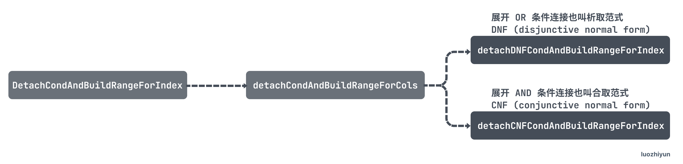
First, DetachCondAndBuildRangeForIndex is called to generate the scan interval, and this function recursively calls the following 2 functions.

detachDNFCondAndBuildRangeForIndex: expands the OR conditional concatenation, also called disjunctive normal form DNF (disjunctive normal form), to generate scan intervals or merge scan intervals.

detachCNFCondAndBuildRangeForIndex: expand AND conditional concatenation also called collocation paradigm CNF (conjunctive normal form), generating scan intervals or merging scan intervals.

The expression tree above eventually generates the interval: [5,12).

Then physicalOptimize recursively calls the findBestTask function for all operators, and finally calls the DataSoure operator to use the Skyline-Pruning index trimming, which gets the optimal execution plan from possibleAccessPaths.

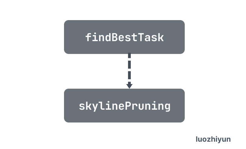
The different physical implementations corresponding to the logical operators differ in terms of time complexity, resource consumption and physical properties. In this process, the optimizer determines the cost of different physical implementations based on statistical information about the data and selects the physical execution plan with the lowest overall cost.

If an execution plan contains multiple indexes, then Skyline-Pruning determines the merit of an index by.

• How many access conditions are covered by the index’s columns. “Access conditions” refers to where conditions that can be translated into a range of columns, and if an index has more access conditions covered by its set of columns, then it is better in this dimension.
• Selects whether the index requires a table lookup when reading tables (i.e., whether the index generates an IndexReader or IndexLookupReader plan). Indexes that do not require a table lookback outperform indexes that require a table lookback in this dimension. If both require table returns, compare how many filter conditions are covered by the index’s columns. Filter conditions refer to where conditions that can be determined based on the index. If the more access conditions are covered by the set of columns of a given index, the fewer table returns it has, the better it is on this dimension.
• Choose whether the index can satisfy a certain order. Because index reads can guarantee the order of certain sets of columns, indexes that satisfy the order required by the query are better in this dimension than indexes that do not.

After using the Skyline-Pruning rule to exclude unsuitable indexes, the selection of indexes is based solely on cost estimation, and the cost estimation of read tables needs to consider the following aspects.

• The average length of each row of data at the storage level for the index.
• The number of rows in the query range generated by the index.
• The table return cost of the index.
• Number of ranges for index queries.

Based on these factors and the cost model, the optimizer selects an index with the lowest cost for table reads.

A structure called task is returned after the final execution, and TiDB’s optimizer will package the PhysicalPlan as a Task.

Currently, TiDB computation task is divided into two different kinds of task: cop task and root task. cop task is the computation task executed by using Coprocessor in TiKV, and root task is the computation task executed in TiDB.

Transactions

Percolator Distributed Transactions

TiDB’s transaction model follows Percolator’s transaction model.

So let’s talk about Percolator distributed transactions first. Percolator

Percolator implements distributed transactions based on three entities: Client, TSO, and BigTable.

• Client is the initiator and coordinator of transactions
• TSO provides an accurate, strictly monotonically incremental timestamp service for distributed servers.
• BigTable is a Google implementation of a multi-maintainer persistent Map.

When Percolator stores one column of data, it stores multiple columns of data in the BigTable: the

• data column (D column): stores value
• lock column (L column): stores lock information for distributed transactions
• write column (W column): stores commit_timestamp for distributed transactions

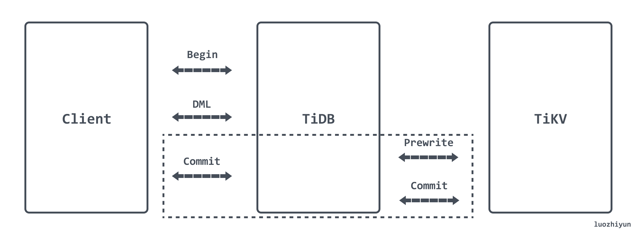
Percolator’s distributed write transaction is implemented by 2-phase commit (later called 2PC). However, it has some modifications to the traditional 2PC. When a write transaction transaction is opened, the Client gets a timestamp from the TSO as the start time of the transaction (later called start_ts). Until commit, all write operations are simply cached in memory. A commit goes through a prewrite phase and a commit phase, and a write transaction can contain multiple write operations.

Write Operations

Prewrite

1. Get a timestamp from TSO as start_ts when the transaction is opened;
2. select one of the write operations for all rows as primary (not only a means of conflict security in itself, but also a marker for resolving the state of the transaction), and the others as secondaries.
3. write the primary row to the L column, i.e., lock it, and check for conflicts before locking.
   1. check whether the L column has already been locked by another client, directly Abort the entire transaction.
   2. check whether the W column has been committed after the start time of the transaction, check the W column, whether there is an update between [start_ts, +Inf) whether there is the same key data. If there is, then there is a conflict in the W column, directly Abort the entire transaction; 4.
4. if there is no conflict, then lock and use start_ts as the Bigtable timestamp to write the data to the data column, which is not visible to other transactions because the write column has not been written yet.

Commit

If Prewrite is successful, proceed to Commit phase.

1. obtain a timestamp from the TSO as the commit time of the transaction (later called commit_ts).
2. commit the primary, and if it fails, abort the transaction.
3. check whether the lock on primary still exists, and abort if it does not. (Other transactions may assume that the current transaction has failed and thus clean up the current transaction’s lock).
4. with commit_ts as timestamp, write to column W, value as start_ts, clean up the data in column L. Note that at this point for Commit Point, “write column W” and “clean up column L” by BigTable’s single-row transaction to ensure ACID.
5. Once the primary commit succeeds, the entire transaction succeeds. At this point, the client can already return success, and then asynchronously secondary commit. seconary commit does not need to detect whether the lock column lock still exists, it will not fail.

Read operation

1. check if the row has an L column with timestamp [0, start_ts], if it does, it means that another transaction is currently occupying the row, try to clear it if this lock has timed out, otherwise wait for the timeout or for another transaction to initiate the unlock.
2. if the lock is found not to exist in step 1, it is safe to read.

TiDB two-phase commit transaction

TiDB commit transactions are performed by calling the Commit method of KVTxn. Like the protocol described in the pecolator paper, this is a two-phase commit process, a Prewrite phase and a Commit phase.

Prewrite:

1. TiDB selects a Key from the current data to be written as the Primary Key for the current transaction.
2. TiDB gets the write route information of all the data from PD and classifies all the Keys according to all the routes. 3.
3. TiDB concurrently issues prewrite requests to all the TiKVs involved, TiKV receives the prewrite data, checks the data version information for conflicts and expiration, and locks the data if it meets the conditions, and records the start time stamp of this transaction in the lock. , delete the data with version startTs.
4. TiDB receives all prewrite successes.

When the Prewrite phase completes, it enters the Commit phase, where the current timestamp is commitTs and TSO ensures that commitTs > startTs.

Commit:

TiDB initiates the second stage commit operation to TiKV where the Primary Key is located. After TiKV receives the commit operation, it checks the data legitimacy and cleans up the locks left in the prewrite stage.

Storage of data

TiDB’s storage layer is implemented by TiKV, which can be seen as a huge Map, that is, it stores Key-Value pairs, in which the Keys are arranged in the order of the total raw binary bits of the Byte array in comparison.

TiKV stores the data in RocksDB, and RocksDB is responsible for the specific data landing. However, RocksDB is a local storage solution, as a distributed storage, it needs to ensure that data will not be lost and error-free in case of single machine failure, so TiKV uses Raft to do data replication, each data change will be landed as a Raft log, and through Raft’s log replication function, data will be synchronized to most nodes of the Group safely and securely.

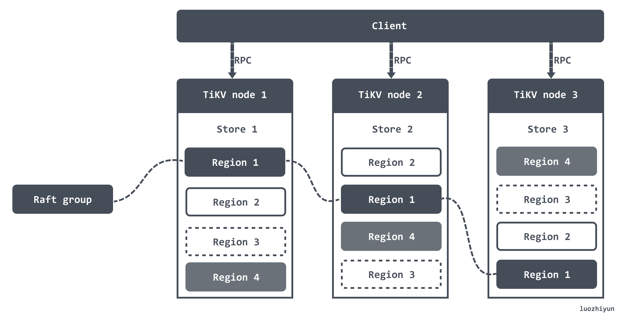
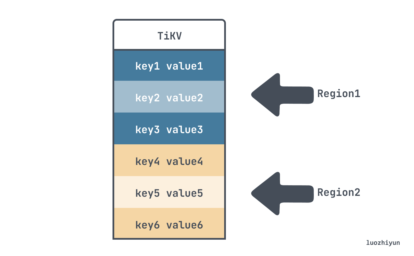
TiKV divides the entire Key-Value space into many segments, each segment is a series of consecutive Keys, we call each segment a Region, and we try to keep the data stored in each Region within a certain size. Each Region can be described by a left-closed-right-open interval like StartKey to EndKey.

After dividing the data into Regions, we will spread the data across all the nodes in the cluster by Region, and try to ensure that the number of Regions served on each node is about the same, and then do the replication and membership management of Raft by Region.

Cluster Availability & Data Consistency Assurance

To achieve cluster and data assurance, we need to collect information, that is, we need to know the status of each TiKV node and the status of each Region.

In simple terms, first information is collected, then scheduling is generated based on the collected information, and finally scheduling is executed.

For information collection, TiKV proactively reports two types of messages to PD periodically.

• Each TiKV node will periodically report the overall information of the node to the PD. This information includes the total disk capacity of the TiKV node, the available disk capacity, the number of Regions hosted, whether it is overloaded, etc.
• The Leader of each Raft Group will periodically report information to the PD. This information is mainly Raft-related, such as the location of the Leader, the location of Followers, the number of fallen Replica, etc.

The PD continuously collects information about the whole cluster through these two types of heartbeat messages, and then uses this information as the basis for decision making to generate a scheduling plan.

For example, if the PD finds that the number of replicas in a region does not meet the requirement through the heartbeat packet of a region leader, it needs to adjust the number of replicas through Add/Remove Replica operation. Then you can use this information to determine whether a node is offline or the administrator has adjusted the replica policy.

In addition to the above issue of Replica number, there are also issues such as: making the number of Leaders evenly distributed among Stores, replicas evenly distributed among Stores, and the number of access hotspots evenly distributed among Stores, and so on.

Finally, according to the scheduling information, the scheduling policy is sent to TiKV’s Region Leader for execution. It should be noted that the scheduling policy here is only a suggestion to the Region Leader, and it is not guaranteed to be executed.

Key-Value Mapping Data

Since TiDB is stored via TiKV, but a table may have many columns in a relational database, it is necessary to map the data of each column in a row into a (Key, Value) key-value pair.

TiDB assigns a TableID to each table, an IndexID to each index, and a RowID to each row (if the table has an integer Primary Key, the value of the Primary Key is used as the RowID), where the TableID is unique within the cluster and the IndexID/RowID is unique within the table, and these IDs are all int64 types.

They are encoded into Key-Value pairs according to the following rules.

1
2

Key: tablePrefix{tableID}_recordPrefixSep{rowID}
Value: [col1, col2, col3, col4]

Unique Index data is encoded into Key-Value pairs according to the following rules.

1
2

Key: tablePrefix{tableID}_indexPrefixSep{indexID}_indexedColumnsValue
Value: rowID

A normal secondary index is encoded as a Key-Value pair according to the following rules.

1
2

Key: tablePrefix{tableID}_indexPrefixSep{indexID}_indexedColumnsValue_rowID
Value: null

For example, there is a table like this.

1
2
3
4
5
6
7
8

CREATE TABLE User (
    ID int,
    Name varchar(20),
    Role varchar(20),
    Age int,
    PRIMARY KEY (ID),
    KEY idxAge (Age)
);

There are three rows of data in the table.

1
2
3

1, "TiDB", "SQL Layer", 10
2, "TiKV", "KV Engine", 20
3, "PD", "Manager", 30

For primary keys and unique indexes, the unique ID of the table and the RowID of the data in the table will be added to each entry, such as the three rows of data above.

1
2
3

t10_r1 --> ["TiDB", "SQL Layer", 10]
t10_r2 --> ["TiKV", "KV Engine", 20]
t10_r3 --> ["PD", "Manager", 30]

Where t in key means TableID prefix, t10 means the unique ID of table is 10; r in key means RowID prefix, r1 means this data RowID value is 1, r2 means RowID value is 2 and so on.

For ordinary secondary indexes that do not need to satisfy the uniqueness constraint, a key value may correspond to multiple rows, and you need to query the corresponding RowID according to the key range. idxAge index in the above data will be mapped to.

1
2
3

t10_i1_10_1 --> null
t10_i1_20_2 --> null
t10_i1_30_3 --> null

The above key corresponds to: table ID_i index ID_index value_RowID.