A short, straightforward introduction to modern processor microarchitecture design.
Today’s robots are very primitive, capable of understanding only a few simple instructions such as ‘go left’, ‘go right’ and ‘build car’.
Warning 1: This article is intended to be about serious science in informal and witty terms.
Warning 2: Long article! Estimated reading time is 36 minutes.
This article introduces some concepts about processor microarchitecture to junior computer science students and readers interested in modern processor architecture. Specifically, there are the following aspects.
- Streamlining (superscalar execution, chaotic execution, very long word instructions, branch prediction)
- Multicore and Hyper-Threading (Synchronous Hyper-Threading SMT)
- SIMD instruction set (SSE, AVS, NEON, SVE)
- Cache and cache mechanism
Sounds like a lot of deep content, but don’t be afraid! This article will take you on a quick tour of what seems like something only a processor design practitioner or architecture expert could understand. Maybe you’ll be able to brag to your classmates/friends soon.
Super 10G
The higher the main frequency, the better the CPU performance, which seems to be a misconception of many people (excluding the up owner quoted above), but, since the ancient times, CPU performance and main frequency are not directly related. So where did this stereotype come from?
Let’s take a look at some upper ancient (late 1990’s) processor data…
| Main Frequency | Model | SPECint95 | SPECfp95 |
|---|---|---|---|
| 195 MHz | MIPS R10000 | 11.0 | 17.0 |
| 400 MHz | Alpha 21164 | 12.3 | 17.2 |
| 300 MHz | UltraSPARC | 12.1 | 15.5 |
| 300 MHz | Pentium II | 11.6 | 8.8 |
| 300 MHz | PowerPC G3 | 14.8 | 11.4 |
| 135 MHz | POWER2 | 6.2 | 17.6 |
SPEC was a commonly used performance test tool back in the day, and Steve Jobs demonstrated the performance improvement of SPEC at the launch when he announced the switch of Apple’s Macbook from IBM PowerPC platform to Intel’s Core platform.
From the table, you can see why there is such a different performance difference for 300MHz processors. Why do the lower main frequency CPUs crush the higher main frequency ones instead?
What? You say this is all the data from the past? Then let’s have a recent one.
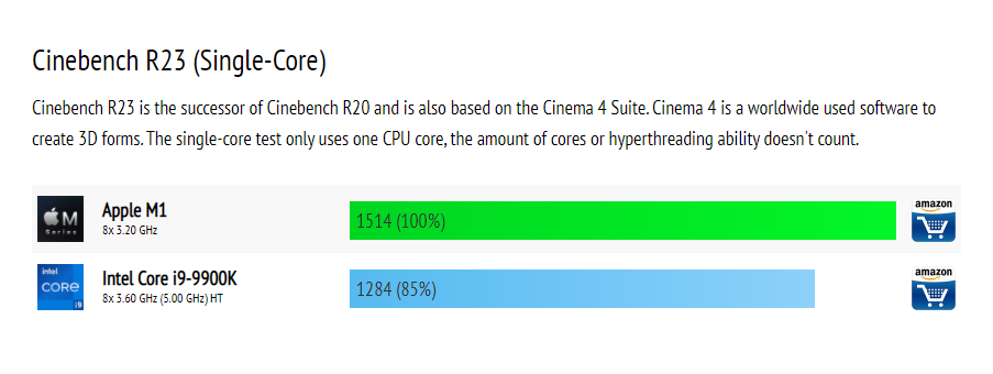
The Intel i9-9900K that is super to half human thank you (5GHz) is actually being hung by the M1?
Yes, you read that right, which means there’s obviously something besides the main frequency, and that is -
Streamline and instruction-level parallelism
Instructions are executed one after the other in the processor, right? Not exactly right. Such a statement may be intuitive, but it is not true. In fact, since the 1980s, CPUs no longer execute each instruction exactly sequentially. Modern processors can execute different stages of different instructions at the same time, and some can even execute multiple instructions completely simultaneously.
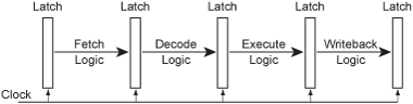
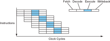
Let’s take a look at how a simple four-stage pipeline is constructed. Instructions are divided into four parts: fetch, decode, execute, and write back .
If the CPU executes fully sequentially, then each instruction takes 4 cycles to execute, IPC = 0.25 (Instruction per cycle). Of course, CPI was preferred in older times, when processors were generally unable to execute one instruction per cycle. But times have changed, and any desktop processor you can get your hands on can execute one, two, or even three instructions in one cycle.
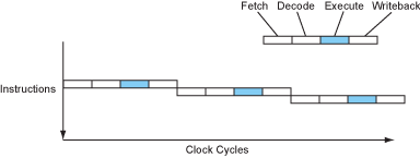
As you can see, the components within the CPU that are responsible for computing (ALU) are actually very laid back, even working only 25% of the time. What? I see you have a talent for capitalism…
Well, modern processors do have the means to squeeze these ALUs (yes, modern processors have more than one ALU too). A very intuitive idea is that since most of the stages are not fully occupied by the CPU, it would be nice to overlap them. Indeed, that’s what modern processors do.
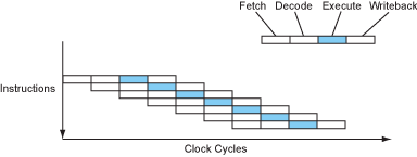
Now we have a processor that can execute one instruction a cycle most of the time, which looks good! That’s already a quadruple speedup without increasing the main frequency.
From a hardware point of view, each stage of the pipeline is made up of logic modules for that stage, and the CPU clock acts like a pump, pumping signals (or one could say data) from one stage to the next one at a time, like this.
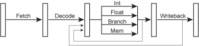
In fact, in addition to such a simple structure, modern processors have, first, many additional ALUs, such as integer multiplication, addition, bitwise operations, various operations on floating-point numbers, etc., with at least one ALU for almost every common operation. second, if the result of the previous instruction is the operand of the next instruction, then why write the data back to the register? Thus comes the Bypass (forward pass) path, used in this case to redirect data to the input port of the operator. Putting it all together, a more detailed pipelined microarchitecture would look like this.
A deeper pipeline - a super pipeline
Since CPU main clock for some reason (some mysterious force?) Since there has been no major improvement for many years (yes, the top of the overclocking list is still AMD’s bulldozer architecture CPU), pipeline design has become almost the race home for CPU manufacturers. Deeper pipelines firstly continue to increase the actual IPC (the theoretical upper limit is still 1), and secondly avoid the impact of pipelines on timing. This has to do with the characteristics of transistors, and interested readers can search the web to find out why multi-stage pipeline structure affects timing and the final synthesis out of the main frequency.
This race reached its peak between 2000-2010, when processors could even have pipelines of up to 31 stages. But the ultra-deep pipeline brought structural complexity and significantly more difficulty in designing dynamic scheduling modules, so there have not been any CPUs with that many pipeline stages since then. For comparison, most current (2021) processors use pipelines ranging from 10-20 levels depending on the application scenario.
x86 and other CISC processors typically have deeper pipelines because they have several times as many tasks to do in the fetch and decode phase, so they typically use deeper pipelines to avoid performance loss in this phase.
Multi-emission - superscalar processors
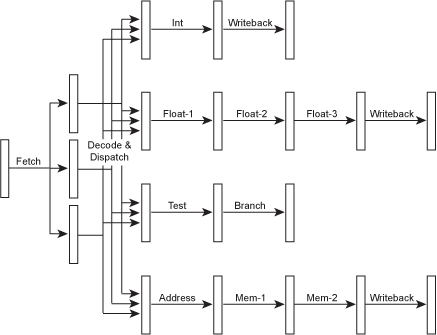
Since integer operators and floating point operators and some other ALUs are not dependent on each other and do their own thing, why not squeeze them further and make them as busy as possible together? This gives rise to multi-launch and superscalar processors. Multi-emission means that the processor can “fire” more than one instruction per cycle, for example, floating-point and integer instructions can be executed simultaneously without interfering with each other. To accomplish this, the logic of the fetch and decode phases must be enhanced, which gives rise to a structure called a scheduler or distributor, which looks like this.
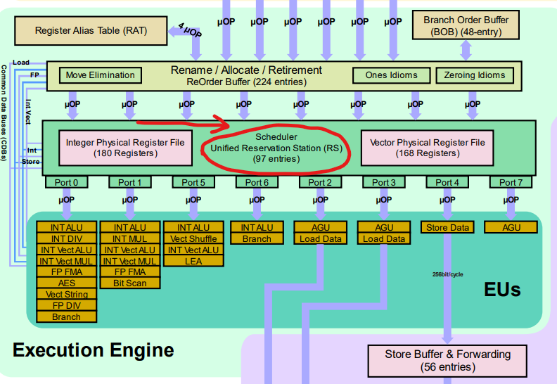
Or let’s look at an actual Intel Skylake architecture scheduler. The red circle in the diagram is the scheduler responsible for “firing” instructions per cycle.
Of course, different operations now have different “data paths” and go through different operators. Because different operators may also have different execution stages within them, different instructions have different pipeline depths: simple instructions are executed faster and complex instructions are executed slower, which reduces the latency of simple instructions (which we’ll get to shortly). Some instructions (such as division) can be quite time-consuming and may take tens of cycles to return, so these factors become especially important in compiler design. The interested reader may wish to consider the usefulness of Mason primes here.
The instruction flow in a superscalar processor might look like this.
Modern processors generally have a considerable number of launch ports, for example, the Intel Skylake mentioned above is an eight-launch architecture, Apple’s M1 is also eight-launch, and ARM’s latest release, the N1, is a 16-launch processor.
Explicit parallelism - extra-long instruction set
When compatibility is not an issue (which, unfortunately, is rarely the case), we can design an instruction set that explicitly states that certain instructions can be executed in parallel, thus avoiding tedious dependency checks at decode time. This would theoretically make the hardware design of the processor simpler, smaller, and easier to achieve higher main frequencies.
In this type of instruction set, an “instruction” is actually a “set of sub-instructions”, which allows them to have a very large number of instructions, and thus each instruction is very long, e.g. 128bits, which is where the name Very Long Instruction Set (VLIW) comes from.
The instruction flow of a Very Long Instruction Set processor is very similar to that of a superscalar processor, except that it eliminates the cumbersome fetch and decode stages, like this.
Except for the hardware architecture, very long instruction set processors are very similar to superscalar processors, especially from the compiler’s point of view (which we will also talk about soon).
However, very long instruction set processors are usually designed to not check dependencies, which makes them dependent on compiler magic to guarantee correct results, and if a cache miss occurs, they have to stop the whole processor, not just the instruction that encountered the cache miss problem. The compiler inserts “nops” (no operations) - that is, empty instructions - between instructions to ensure that data-dependent instructions are executed correctly. This undoubtedly makes the compiler more difficult to design and takes longer to compile, but it also saves valuable on-chip processor resources and often results in slightly better performance.
Intel’s IA-64 architecture was a very long instruction set (VLIW) architecture, and the resulting “Itanium” family of processors was considered the successor to x86 at the time. The “Itanium” series of processors was considered the successor to the x86 at the time, but the market did not like the new architecture, so the series did not develop. The hottest direction of modern hardware acceleration is the GPU, which can also be considered a VLIW architecture processor, but it takes the VLIW architecture a step further by using “core functions” instead of instructions, which greatly increases the scalability of this architecture, and is also available to interested readers.
Data dependency and latency
How far can we go down the road of pipelining and multi-launching? If multi-launch and multi-stage pipelining are so good, why not make a 50-stage pipelined, 30-launch processor? Let’s discuss the following two instructions.
Second instruction Dependent First instruction - the processor cannot execute the next instruction until it has completed the previous one. This is a serious problem, which makes multiple firing useless, because no matter how many firing processors you make, the two instructions can still only be executed sequentially (excluding parts such as fetching fingers). We will discuss about dependencies and elimination later.
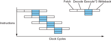
If the first instruction is a simple addition instruction, then the adder can pass the data back to the input port of the ALU via the Bypass path (forward pass) after execution and continue the computation so that the pipeline can work properly. But unfortunately, the first instruction is a multiplication that requires multiple cycles to complete (most current CPUs do not use single-cycle multiplication because the complex logic usually hurts the main frequency), so the processor has to add a number of “bubbles” to the pipeline in order to wait for the first instruction to complete, which is similar to “nops” to ensure the correctness of the operation.
The number of CPU cycles it takes between the time an instruction reaches the input port of the operator and the time the result is available for execution is called instruction latency. The deeper the pipeline, the higher the instruction latency, so a deeper pipeline that cannot be filled efficiently will only result in high instruction latency without any benefit to the processor performance.
From the compiler’s point of view (taking into account Bypass, the latency in the hardware engineer’s mouth usually does not include Bypass), the instruction latency of modern processors is typically: 1 cycle for integer multiplication and bit operations, 2-6 cycles for floating point multiplication and addition, 10+ cycles for complex instructions like sincos, and finally division which can be up to 30-50 cycles.
The latency of access operations is also a very problematic issue, because they are usually the very first step of each instruction, which makes the latency they cause difficult to compensate in other ways. In addition to this, their latency is also hard to predict, because the latency depends heavily on whether the cache hits or not, and the cache is dynamically scheduled (which we will also talk about soon).
Branching and branch prediction
Another important issue in the pipeline is branching, so let’s look at the next section of the program.
The compiled assembly program will look like this.
Now imagine a pipelined processor executing this program. By the time the processor reaches the second line, that is, the second line of the jump command, the processor’s executor must have removed all subsequent instructions from memory in advance and completed the decoding process. But which instruction is being jumped? Is it line 3, line 4 or line 5? We don’t know where to jump until the jump command reaches the executor. In a deeply pipelined processor, it seems to have to stop and wait for the jump command, then refill the pipeline with new instructions. This is of course unacceptable. Programs, especially loops, have a large percentage of branch-jump commands, and if we waited for this command to complete every time, then our pipeline would have to pause frequently, and the performance gains we achieved with the pipeline would be lost.
So modern processors make guesses . What? I thought the advanced processor design industry could come up with a better solution! Don’t worry yet, there is actually a pattern to the branch jumps in the program, and modern processors branch predictions are typically 99% accurate or better (although branch predictions are also the source of Intel’s spectre and meltdown vulnerabilities).
The processor will execute along the predicted branch , so that our processor can keep the pipeline and operators occupied and execute at high speed. Of course, the result of the execution is not yet final; only after the result of the branch-hopping command is available will the correct prediction be written back (commit or retire). What about wrong guesses? Then the processor has no choice but to start the pipeline again from another branch, and in highly streamlined modern processors, the cost of a branch prediction error (branch prediction error penalty) is quite high, often amounting to tens of CPU cycles.
The key here is how processors make predictions. In general, there are two types of branch prediction: static and dynamic.
Static branch prediction means that the processor makes a guess independent of the runtime state and the optimization of the jumps is done by the compiler. Static predictions usually have a blanket jump or a backward jump that predicts no jump, and a forward jump that predicts a jump. The latter usually works better because loops generally have a large number of forward jump instructions in them.
Dynamic branch prediction, on the other hand, decides whether to jump or not based on the history of jump instructions . One of the simplest dynamic branch predictors is the 2-bit saturation counter , which is a four-state state machine characterized by the fact that only two consecutive prediction errors will change the prediction direction. It has been able to achieve more than 90% correct prediction rates in most settings.
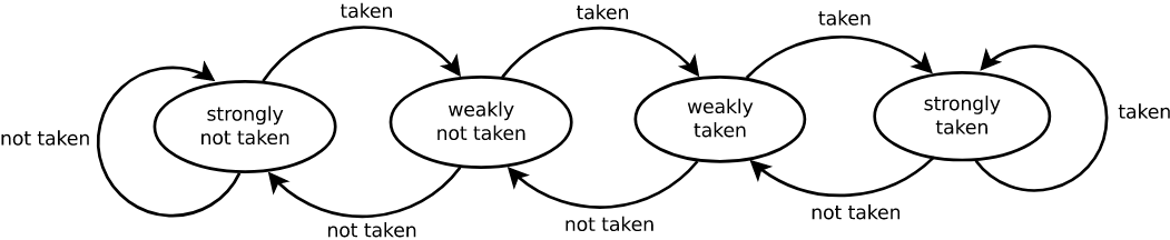
This predictor performed poorly when alternating jump and non-jump branch instructions, so the n-level adaptive branch predictor was invented, which is similar in principle to a 2-bit saturation counter, although it can remember the past n histories and perform well in repeated jump patterns.
Unfortunately, branch prediction is one of the core competencies of each CPU vendor, and most good branch prediction techniques are also important trade secrets, so there is not much to dive into in this area. cloudflare recently published a blog post that tested in depth the characteristics of branch predictors on M1 for x86 and ARM, and interested readers can take a look.
Removing Branching Statements
Since branching is something that processors don’t like, people want to minimize the use of branch statements. The following is common, and is often used when finding the maximum and minimum values or when making conditional assignments (lines 1, 2).
So people devised instructions like line 3. Such an instruction assigns the value of d to b under a specific condition without introducing a branch, and simply does not write back (commit/retire) when the condition is not satisfied. This instruction is called a conditional transfer instruction and is often used in compilers to avoid jumping.
Our ancient x86 architecture did not support conditional transfer instructions to begin with, nor did MIPS or SPARC, while the Alpha architecture was designed from the beginning with such instructions in mind (newer instruction sets like RISC-V certainly do.) ARM, on the other hand, was the first instruction set to use fully predictable instructions, which is interesting because early ARM processors typically used a very shallow pipeline with The branch prediction penalty was very small.
Instruction Scheduling, Register Renaming, and Chaotic Execution
If branches and long-latency instructions introduce pipeline bubbles, can the processor time taken up by these bubbles be used for useful things? To achieve this, it is necessary to introduce random execution . Chaotic execution allows the processor to disorder some of the instructions and execute something else at the same time as the long latency instructions.
Historically, there have been two ways to achieve chaotic execution: software and hardware.
The software approach is well understood and involves strong compiler-architecture coupling to generate instructions at the compile stage that are free of interdependencies and easy to schedule by the processor. The advantage of instruction rescheduling at the compile stage, also known as static instruction scheduling, is that the software implementation can be more flexible (as we all know, software can do anything), and often the software can also have enough storage space to analyze the entire program and therefore obtain a better instruction layout. The disadvantages are of course obvious, as the compiler requires in-depth knowledge of architecture-related information, such as instruction latency and branch prediction penalties, making portability very difficult. Therefore the hardware approach is more commonly used in modern processors.
The hardware approach focuses on register renaming to eliminate read-read and write-write pseudo-dependencies. Register renaming means using different physical hardware storage for the same registers called by different instructions, and then sorting these instructions and registers in the write-back phase so that these false dependencies are no longer the cause of pipeline bubbles. Note that write-read dependencies are true data dependencies, and while techniques like forward delivery can reduce latency, there is no solution to such dependencies. Modern processors also do not have just 16 general-purpose registers and 32 floating-point registers, for example, but usually hundreds of physical registers on the CPU’s chip. The most famous algorithm for register renaming is the Tomasulo algorithm, which the interested reader can search for.
The advantage of the hardware approach is that it reduces the architecture coupling of the compiler, improves the convenience of software writing, and usually the hardware messy execution is not as bad as the software. The disadvantage is that both dependency analysis and register renaming consume valuable on-chip space and power, but the performance improvement is not correspondingly large. Therefore, sequential execution is used in some CPUs that are more concerned with low power consumption and cost, such as ARM’s low-power product line, Intel Atom, etc.
Multicore and Hyper-Threading
We have previously discussed various approaches to instruction set parallelism, and many times they do not work very well because a significant portion of programs do not provide fine-grained parallelism. Therefore, the effect of making wider and deeper processors is quite limited.
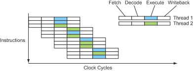
But then the CPU designers thought, if there is no sufficient parallelism in this program without interdependent instructions, then there must be no data dependency between different programs (instruction-level data dependency), so wouldn’t it be nice to run two threads on the same physical core at the same time to fill in the gaps in the pipeline with each other? This is called synchronous multithreading (SMT) , and it provides thread-level parallelization. This technique is transparent to the world outside the CPU, as if there were really twice as many CPUs, hence the virtual cores that are now also often spoken of.
From a hardware perspective, a synchronous multithreading implementation requires doubling the number of all structures related to running state, such as registers, PC counters, MMUs and TLBs, etc. Fortunately, these structures are not a major part of the CPU, and the most complex decoders and distributors, operators and caches are shared between the two threads.
Of course, the real performance cannot be doubled, the theoretical upper limit depends on the number of operators, and synchronous multithreading just makes better use of the operators. Therefore, in tasks such as game screen generation, where parallelism is already very high, SMT has almost no effect, but instead brings some performance loss due to occasional thread switching.
The instruction flow of the SMT processor looks something like this.
Great! Now we have a way to fill which pipeline bubbles, without any risk. So, 30-launch processor here we come! Is that right? Unfortunately, no.
Although IBM has used 8-threaded cores in its products, but we will soon see that the bottleneck of modern processors has long been not only the CPU itself, access memory latency and bandwidth have become more urgent issues to solve. And using 8 MMUs, 8 PCs, and 8 TLBs at the same time is not a cache-friendly approach. As a result, it is rare to hear of processors with more than one core and two threads anymore.
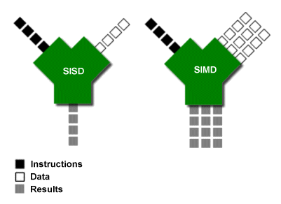
Data parallelism - SIMD instruction set
In addition to instruction-level parallelism and hyperthreading, there is another type of parallelized design in modern processors - data parallelization. The idea of data parallelization is to parallelize different data of the same instruction, not to parallelize different instructions. That is why instruction sets that use data parallelization are often called SIMD instruction sets (single instruction multiple data) or vector instruction sets.
In supercomputers and high performance computing, SIMD instruction sets are used extensively because scientific computations usually deal with extremely large amounts of data without complex operations on each piece of data and with essentially no interdependencies. The SIMD instruction set is also present in a large number of modern personal computers, even in the most inexpensive cell phones.
The SIMD instruction set works as shown in the following diagram.
Intel has been increasing the length of vectors that can be parallelized over the past 20 years, from 128bits for SSE to 512bits for AVX512, while ARM has leaped from 128bits for NEON to 2048bits for SVE since ARMv8a. ARM has leaped from NEON’s 128bits to SVE’s 2048bits since ARMv8a, and even supports variable length.
Modern x86-64 processors support the SSE instruction set, so compilers now automatically add the SSE instruction set for optimization if they compile target files for 64-bit platforms. Because the SIMD instruction set is evolving rapidly, many instructions have latencies comparable to traditional scalar commands, and because the SSE instruction set also has instructions that operate on individual operands, modern compilers use the SSE instruction set by default for individual floating-point operations instead of using traditional x87 floating-point instructions. In addition, almost all architectures have their own SIMD instruction set.
Simple and repetitive tasks like rendering screens or scientific calculations are well suited to the SIMD instruction set, and in fact, GPUs work similarly to SIMD. Unfortunately, the SIMD instruction set does not work well in most ordinary (unthought-out) code. Modern compilers all have varying degrees of automatic loop vectorization (using the SIMD instruction set), but when the program writer does not give good consideration to data dependencies and memory layout (as will be discussed shortly), the compiler often fails to optimize the code much. Fortunately, it is often possible for the compiler to understand that certain loops can be optimized with simple changes, which in turn can dramatically improve the speed of the program.
Memory and memory walls
Modern processors are so fast that they spend most of their time waiting for memory to respond instead of doing their job.
– Anonymous (forgot the source)
Since the invention of computers, processors have evolved much faster than storage, as shown in the following comparative chart.
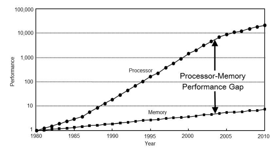
Memory access is very expensive for modern processors.
- In 1980, a CPU access to memory typically took only one cycle.
- In 2021, it will take about 300-500 cycles for a CPU to access memory.
When we consider that we use so many means on the CPU to squeeze the operators so that the IPC can break 1, this makes memory even slower to look at. Here is a table showing how long it takes to access the rest of the memory if the processor cycle is considered as 1 second.
| Event | Delay | Equivalent Delay |
|---|---|---|
| CPU cycles | 0.2ns | 1s |
| L1 cache access | 0.9ns | 4s |
| L2 cache access | 3ns | 15s |
| L3 cache accesses | 10ns | 50s |
| Memory access | 100ns | 8min |
| Solid-state drive access | 10-100us | 15-150h |
| mechanical hard drive access | 1-10ms | 2-18 months |
As you can see, modern CPUs are simply too fast and programmers now have to spend more effort than in the past to make their programs take full advantage of the CPU’s performance instead of getting stuck on memory operations.
To solve this serious problem, processor designers have come up with a solution, the cache that has appeared in the table above. 80s CPUs were basically not designed with a cache because there was no memory wall problem. Modern CPUs generally have up to three levels of cache (some low-power and mobile CPUs have only two), and understanding how these caches work is good for programmers to write faster programs.
Cache
Modern processors use multiple levels of cache to avoid the effects of memory latency in order to address memory walls. A typical cache structure looks like this.
| level | size | delay | physical location |
|---|---|---|---|
| L1 cache | 32 KB | 4 cycles | internal per core |
| L2 cache | 256 KB | 12 cycles | per die or per core |
| L3 cache | 6 MB | ~21 cycles | shared across the processor or per die |
| RAM | 4+ GB | ~117 cycles | on a memory stick on the motherboard |
Happily, the caching mechanisms of modern processors are surprisingly effective, with L1 cache hit rates as high as 90% most of the time, indicating that the cost of a memory access is only a few cycles in most cases.
The cache is able to achieve such good results mainly because the program is well localized. There are spatial locality and temporal locality. Time-locality means that when a program accesses a piece of memory, it is likely to access that piece of memory consecutively next. Spatial locality means that when a program accesses a piece of memory, it is likely to access a nearby piece of memory perhaps. To take advantage of such locality, the data in memory is copied from the memory sticks to the cache piece by piece, and these fast are called cache lines.
From a hardware perspective, the cache works much like a key-value pair table; the Key is the address of the memory, and the Value is the corresponding data. In fact the Key is not necessarily the full address, but is usually a part of the high bit of the address, while the low bit is used to index the cache itself. It is possible to use both physical and virtual addresses as Key, and there are advantages and disadvantages to each (as with all things). The disadvantage of using virtual addresses is that process context switches require cache refreshes, which are very expensive. The disadvantage of using physical addresses is that every time you check the cache, you need to check the page table first. Therefore, modern processors usually use virtual addresses as cache indexes and physical addresses as cache line markers. Such an approach is also known as " virtual index - physical tag" caching.
Cache Conflicts and Relevance
Ideally, caches should hold the most recently used data, but for hardware caches on CPUs, algorithms to efficiently maintain usage state cannot meet strict latency requirements and are difficult to implement in hardware, so usually processors use a simple approach: each cache line corresponds directly to several locations in memory . Since the corresponding locations are unlikely to be accessed simultaneously, the cache is valid.
This is very fast (which is what caches were originally designed for), but when the program does keep accessing different locations corresponding to the same cache line back and forth, the cache control unit has to repeatedly load data from memory, which is very time consuming and is called a cache conflict. The solution is not to limit each memory region to one cache line, but to several, which are called cache associativity.
Of course, the fastest way is to have one cache line per memory region, which is called a direct mapped cache, and a cache using four associativity levels is called a 4-channel associative cache. A cache where memory can be loaded to any cache line is called a full associative cache. The benefit of using associative caching is that it greatly reduces cache conflicts while keeping query latency within a reasonable range. This is also the approach typically used by modern processors.