Tracking rpcx microservices with ebpf

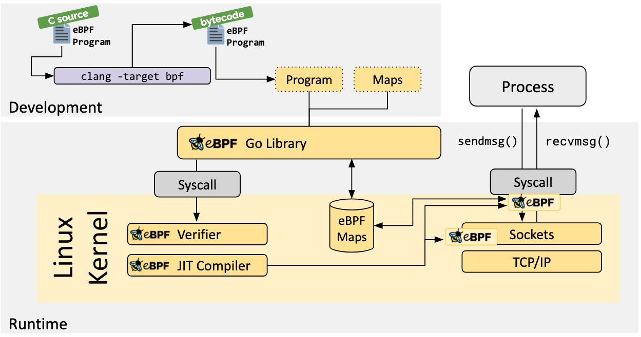
ebpf is an innovative and revolutionary technology that enables sandboxed programs to be run in the kernel without modifying the kernel source code or loading kernel modules. By making the Linux kernel programmable, it is possible to build smarter, more feature-rich infrastructure software based on existing (rather than adding new) abstraction layers, without increasing system complexity or sacrificing execution efficiency or security.

The first version of BPF was introduced in 1994. We actually use it when writing rules using the tcpdump tool, which is used to view or “sniff” network packets.

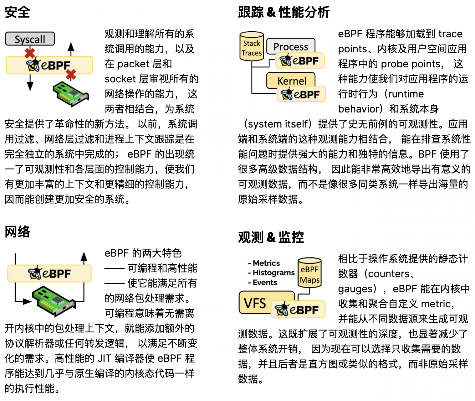
Using ebpf technology, you can provide new ideas and techniques in the direction of security, trace & performance analysis, networking, observation & monitoring, etc.

• Security: You can check security from system call level, packet level, socket level, such as developing DDOS protection system and writing firewall programs.
• Network: You can develop kernel layer high performance packet handler, such as Cilium to provide kernel layer load balancing, and push service mesh to deeper layer to solve sidecar performance problems.
• Trace & Performance Analysis: Linux provides many types of probe points, such as Kernel probes, perf events, Tracepoints, User-space probes, User statically defined tracepoints, XDP and so on. We can write probe programs to collect information about these probe points, so we can track programs and analyze performance in this way.
• Observation & Monitoring: With continuous observation and monitoring of these probe points, we can enrich our trace program. The key is that we do not need to change the established programs, but observe them from other programs through the ebpf method. 2014, Alexei Starovoitov, a famous kernel hacker, extended the functionality of BPF. He increased the number of registers and the allowed size of the program, added JIT compilation, and created a program for checking if the program is safe. Most impressively, however, the new BPF program was able to run not only while processing packets, but also to respond to other kernel events and pass information back and forth between kernel and user space. alexei Starovoitov’s new version of BPF was called eBPF (e stands for extended: extended). But now that it has replaced all older versions of BPF usage and has become so popular, it is still referred to as BPF for simplicity’s sake.

You can write your own bpf programs for custom logic processing and analysis, or you can use tools written by the greats and use them for generic performance analysis and tracing of your programs. This article is about using some tools to do generic analysis of rpcx microservices programs, since they are generic, you can can analyze other Go programs, and not only limited to Go programs, other applications and even kernels you can analyze and trace.

For how to write bpf programs I am going to introduce it in a new article.

This time it will focus on bcc provides related tools and bpftrace.

bcc is a toolkit for creating efficient eBPF-based kernel tracing and manipulation programs, including some useful command line tools and examples. BCC simplifies the writing of eBPF programs for kernel detection in C, including wrappers for LLVM and front-ends for Python and Lua. It also provides high-level libraries for direct integration into applications.

bpftrace is a high-level trace language for Linux eBPF. Its language is inspired by awk and C as well as by previous tracing programs such as DTrace and SystemTap. bpftrace uses LLVM as a backend to compile scripts into eBPF bytecode and uses BCC as a library to interact with the Linux eBPF subsystem as well as existing Linux tracing features and connection points.

Simple rpcx microservice program

Since we are going to use the ebpf analysis program, first we need to have a program. Here I have chosen rpcx a simplest example to implement a minimal microservice for multiplication.

The code of this program can be downloaded at rpcx-examples-102basic.

The server-side program is as follows:

 1
 2
 3
 4
 5
 6
 7
 8
 9
10
11
12
13
14
15
16
17
18
19
20
21
22
23
24
25
26
27

package main
import (
    "context"
    "flag"
    "fmt"
    example "github.com/rpcxio/rpcx-examples"
    "github.com/smallnest/rpcx/server"
)
var (
    addr = flag.String("addr", "localhost:8972", "server address")
)
type Arith struct{}
// 使用ebpf跟踪这个服务调用
func (t *Arith) Mul(ctx context.Context, args example.Args, reply *example.Reply) error {
    reply.C = args.A * args.B
    fmt.Println("C=", reply.C)
    return nil
}
func main() {
    flag.Parse()
    s := server.NewServer()
    s.RegisterName("Arith", new(Arith), "")
    err := s.Serve("tcp", *addr)
    if err != nil {
        panic(err)
    }
    }

Use go build server.go to compile the server program and run it (. /server).

The client application is as follows:

 1
 2
 3
 4
 5
 6
 7
 8
 9
10
11
12
13
14
15
16
17
18
19
20
21
22
23
24
25
26
27
28
29
30
31
32
33
34

package main
import (
    "context"
    "flag"
    "log"
    "time"
    "github.com/smallnest/rpcx/protocol"
    example "github.com/rpcxio/rpcx-examples"
    "github.com/smallnest/rpcx/client"
)
var (
    addr = flag.String("addr", "localhost:8972", "server address")
)
func main() {
    flag.Parse()
    d, _ := client.NewPeer2PeerDiscovery("tcp@"+*addr, "")
    opt := client.DefaultOption
    opt.SerializeType = protocol.JSON
    xclient := client.NewXClient("Arith", client.Failtry, client.RandomSelect, d, opt)
    defer xclient.Close()
    args := example.Args{
        A: 10,
        B: 20,
    }
    for {
        reply := &example.Reply{}
        err := xclient.Call(context.Background(), "Mul", args, reply)
        if err != nil {
            log.Fatalf("failed to call: %v", err)
        }
        log.Printf("%d * %d = %d", args.A, args.B, reply.C)
        time.Sleep(time.Second)
    }
}

The client calls the Arith.Mul microservice once every second, and the logic of the microservice is simple: it performs multiplication and returns the result to the client.

Tracing and analyzing microservices

As a demo, this article only tracks server-side Arith.Mul calls.

bcc provides a number of bpf-based analyzers, as follows (classic diagram put together by Brendan Gregg)

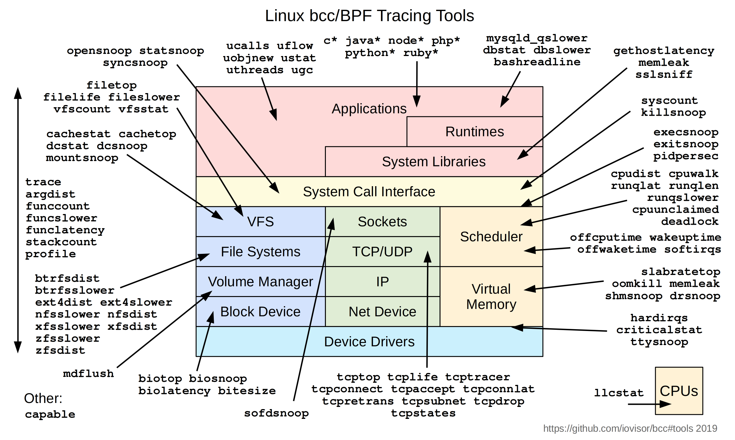
Here we will select a few relevant tools to demonstrate how to use these tools to analyze running programs. Note that it is a running program and we have not added some additional trace points to the program.

bcc package

First you have to install the bcc suite, and your Linux kernel has to be new enough. In some big houses, there are still some kernel versions of 2.6.x servers, and these old kernel servers cannot support ebpf or the new features of ebpf.

I tested this on one of my virtual machines in AliCloud, which is of version:

• Linux lab 4.18.0-348.2.1.el8_5.x86_64
• CentOS Stream release 8

Installing these tools is done directly with yum install bcc-tools.

If you are on a different version of the operating system, you can install them by referring to the bcc installation documentation: bcc/INSTALL.

Before using the tools for analysis, you first need to know the name of your microservice Arith.Mul in the symbol table, which you can query using objdump.

1
2

[root@lab server]# objdump -t server|grep Mul|grep main
000000000075a5e0 g     F .text  00000000000000d0              main.(*Arith).Mul

Its name is main.(*Arith).Mul , and we will use this name to analyze the microservice below.

Make sure that the server you just created is always running.

funccount

funccount is used to count the number of times a function has been called over time.

Execute the following command in the directory where the server is located (if it is in a different path, you need to change the path of the program in the command parameter):

1
2
3
4
5
6

[root@lab server]# funccount -d 10  './server:main.*.Mul'
Tracing 1 functions for "b'./server:main.*.Mul'"... Hit Ctrl-C to end.
FUNC                                    COUNT
b'main.(*Arith).Mul'                       10
Detaching...
[root@lab server]#

Here we set the observation time to 10 seconds, and we can see that this function is called 10 times during these 10 seconds.

It contains several parameters, for example, you can keep observing and output the result every 5 seconds:

1
2
3
4
5

[root@lab server]# funccount -Ti 5  './server:main.*.Mul'
Tracing 1 functions for "b'./server:main.*.Mul'"... Hit Ctrl-C to end.
18:08:29
FUNC                                    COUNT
b'main.(*Arith).Mul'                        5

We can even use it for Go GC related function tracing.

1
2
3
4
5

[root@lab server]# funccount -d 10  './server:runtime.*.gc*'
Tracing 21 functions for "b'./server:runtime.*.gc*'"... Hit Ctrl-C to end.
FUNC                                    COUNT
b'runtime.(*gcControllerState).update'        2
b'runtime.mallocgc'                       250

Or track Go runtime scheduling.

1
2
3
4
5

[root@lab server]# funccount -d 10  './server:runtime.schedule'
Tracing 1 functions for "b'./server:runtime.schedule'"... Hit Ctrl-C to end.
FUNC                                    COUNT
b'runtime.schedule'                        20
Detaching...

funclatency

funclatency counts the time taken by the execution of a function. If we want to analyze the execution of the Arith.Mul method, we can use the following command, which will show the distribution of the time spent on this function call in the form of a histogram.

 1
 2
 3
 4
 5
 6
 7
 8
 9
10
11
12
13
14
15
16
17
18
19
20
21

[root@lab server]# funclatency -d 10  './server:main.*.Mul'
Tracing 1 functions for "./server:main.*.Mul"... Hit Ctrl-C to end.
Function = b'main.(*Arith).Mul' [359284]
     nsecs               : count     distribution
         0 -> 1          : 0        |                                        |
         2 -> 3          : 0        |                                        |
         4 -> 7          : 0        |                                        |
         8 -> 15         : 0        |                                        |
        16 -> 31         : 0        |                                        |
        32 -> 63         : 0        |                                        |
        64 -> 127        : 0        |                                        |
       128 -> 255        : 0        |                                        |
       256 -> 511        : 0        |                                        |
       512 -> 1023       : 0        |                                        |
      1024 -> 2047       : 0        |                                        |
      2048 -> 4095       : 0        |                                        |
      4096 -> 8191       : 0        |                                        |
      8192 -> 16383      : 0        |                                        |
     16384 -> 32767      : 7        |****************************************|
     32768 -> 65535      : 3        |*****************                       |
avg = 31978 nsecs, total: 319783 nsecs, count: 10

We counted 10 seconds of data. You can see that this function was called 10 times during this period. The average time taken is 31 microseconds.

If we want to check if there is a long tail in the online program, it is easy to analyze the statistics using this tool.

funcslower

funcslower This tool can trace functions that execute slowly in the kernel and in the program, for example using the following command.

1
2
3
4
5
6
7

[root@lab server]# funcslower -u 10  './server:main.(*Arith).Mul'
Tracing function calls slower than 10 us... Ctrl+C to quit.
COMM           PID    LAT(us)             RVAL FUNC
server         359284   44.75                0 ./server:main.(*Arith).Mul
server         359284   30.97                0 ./server:main.(*Arith).Mul
server         359284   33.38                0 ./server:main.(*Arith).Mul
server         359284   31.28                0 ./server:main.(*Arith).Mul

You can even print out the stack information:

 1
 2
 3
 4
 5
 6
 7
 8
 9
10
11
12
13
14
15
16
17
18

[root@lab server]funcslower -UK -u 10  './server:main.(*Arith).Mul'
Tracing function calls slower than 10 us... Ctrl+C to quit.
COMM           PID    LAT(us)             RVAL FUNC
server         359284   31.20                0 ./server:main.(*Arith).Mul
    b'runtime.call64.abi0'
    b'runtime.reflectcall'
    b'reflect.Value.call'
    b'reflect.Value.Call'
    b'github.com/smallnest/rpcx/server.(*service).call'
    b'github.com/smallnest/rpcx/server.(*Server).handleRequest'
    b'github.com/smallnest/rpcx/server.(*Server).serveConn.func2'
    b'runtime.goexit.abi0'
server         359284   32.23                0 ./server:main.(*Arith).Mul
    b'runtime.call64.abi0'
    b'runtime.reflectcall'
    b'reflect.Value.call'
    b'reflect.Value.Call'
    b'github.com/smallnest/rpcx/server.(*service).call'

tcp series tools

bcc provides a bunch of tools for tcp tracing, we can use them for different scenarios.

• tools/tcpaccept: Tracks TCP passive connections (accept()).
• tools/tcpconnect: Traces TCP active connections (connect()).
• tools/tcpconnlat: Tracks TCP active connection latency (connect()).
• tools/tcpdrop: Tracks TCP packet drop details for kernel.
• tools/tcplife: Tracks TCP session (lifecycle metrics summary).
• tools/tcpretrans: Tracks TCP retransmissions.
• tools/tcprtt: Tracks TCP round-trip elapsed time.
• tools/tcpstates: Tracks TCP session state changes.
• tools/tcpsubnet: Summarize and aggregate TCP transmissions by subnet.
• tools/tcpsynbl: Displays TCP SYN backlog.
• tools/tcptop: Aggregates TCP send/recv throughput by host.
• tools/tcptracer: Tracks TCP connection creation/closure (connect(), accept(), close()).
• tools/tcpcong: Tracks the duration of TCP socket congestion control state.

For example, if we are concerned about connection establishment, we can use tcptracer:

 1
 2
 3
 4
 5
 6
 7
 8
 9
10
11

[root@lab lib]# tcptracer
Tracing TCP established connections. Ctrl-C to end.
T  PID    COMM             IP SADDR            DADDR            SPORT  DPORT
C  360005 client           4  127.0.0.1        127.0.0.1        43126  8972
X  360005 client           6  [::1]            [::1]            43010  8972
A  359284 server           4  127.0.0.1        127.0.0.1        8972   43126
X  360005 client           4  127.0.0.1        127.0.0.1        43126  8972
X  359284 server           4  127.0.0.1        127.0.0.1        8972   43126
C  360009 client           4  127.0.0.1        127.0.0.1        43130  8972
X  360009 client           6  [::1]            [::1]            43014  8972
A  359284 server           4  127.0.0.1        127.0.0.1        8972   43130

There are also a bunch of xxxxsnoop programs that can be traced for specific system calls.

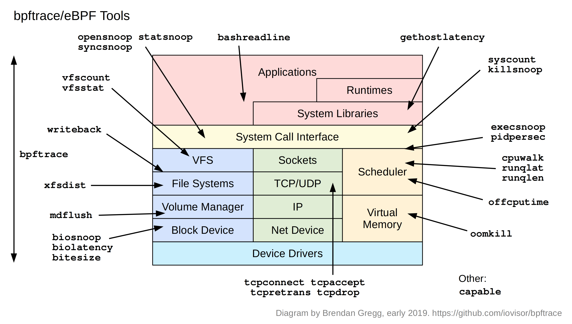
bpftrace

Sometimes we want to implement some custom tracing using scripts, for example tools like awk that provide simple scripting.

One such tool is bpftrace, which uses LLVM as the backend to compile scripts into eBPF bytecode and uses BCC as a library to interact with the Linux eBPF subsystem as well as existing Linux trace functions and connection points.

The bpftrace reference manual can be found at bpftrace reference_guide.

Using our Arith.Mul as an example, we can use the following command to add a probe to the function call to print out the input parameters.

1
2
3
4
5

[root@lab server]# bpftrace -e 'uprobe:./server:main.*.Mul {printf("%s - %s: arg1: %d, arg2: %d\n", comm, func, arg0, arg1)}'
Attaching 1 probe...
server - main.(*Arith).Mul: arg1: 10, arg2: 20
server - main.(*Arith).Mul: arg1: 10, arg2: 20
server - main.(*Arith).Mul: arg1: 10, arg2: 20

Why does arg0,arg1 just print out the parameters? Simply put, our microservice arguments are exactly two int64 integers, which correspond exactly to arg0,arg1.

The service return value of rpcx is also passed in as an argument and has not been set when the function is called, so if you print arg3 is not a REPLY return value.

At this point we need to move the probe and add an offset, how much of an offset do we add? By disassembling we see that the return value has been assigned when adding 92, so use the following command to print the return value (this time the first argument is overwritten).

1
2
3
4
5

[root@lab server]# bpftrace -e 'uprobe:./server:main.*.Mul+92 {printf("%s - %s: reply: %d\n", comm, func, arg0)}'
Attaching 1 probe...
server - main.(*Arith).Mul: reply: 200
server - main.(*Arith).Mul: reply: 200
server - main.(*Arith).Mul: reply: 200

Go has changed to a register-based calling convention since 1.17, so here we use the built-in arg0, arg1,… , if you are using an earlier version of Go, here you can switch to sarg0,sarg1,… Try (stack arguments).