1. Introduction
I believe there is no one who has not used P2P technology. BT seeds and magnetic links are the most common P2P technologies. With P2P technology, files are no longer stored centrally on one server, but are distributed among users’ nodes, each of which is a provider and a user of the service. Such a system has high availability, so that the whole service will not be unavailable due to the downtime of one or two machines. So how is such a system implemented, how is it decentralization and self-organization? In this article, we will discuss this problem.
This article will first introduce the general idea of P2P networks, and introduce the main character of P2P networks - Distributed Hash Table (DHT); then we will introduce two distributed hash table algorithms. These will give you a more concrete understanding of P2P technology.
2. Overview of P2P networks
2.1 Traditional CS networks and P2P networks
CS architecture is a Client-Server architecture, which consists of a server and a client: the server is the service provider and the client is the service user. Many of the applications we use today such as web drives, video applications, online shopping platforms, etc. are CS architectures. Its architecture is shown in the figure below:
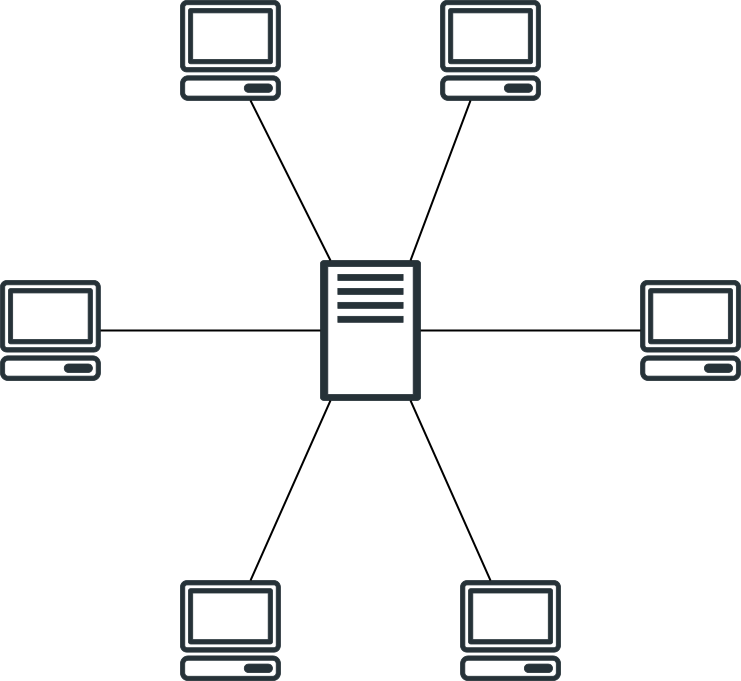
Of course the server is not usually a single point, but often a cluster; but it is essentially the same. The problem with the CS architecture is that once the server is down, for example, by a DDoS attack, the client is no longer available and the service is lost.
To solve this problem, P2P Networking (Peer-to-peer Networking) has been proposed. In P2P networks, there is no longer a central server providing the service, there is no longer the concept of “server”, everyone is a service provider and a service user - i.e., everyone can be a server. Our common BT seed and magnetic link download services are P2P architectures. A P2P system has been defined as follows:
a Peer-to-Peer system is a self-organizing system of equal, autonomous entities (peers) which aims for the shared usage of distributed resources in a networked environment avoiding central services.
A P2P system is a self-organizing system in which each node is equal, autonomous, and aims to share the use of distributed resources in a network environment that avoids centralized services.
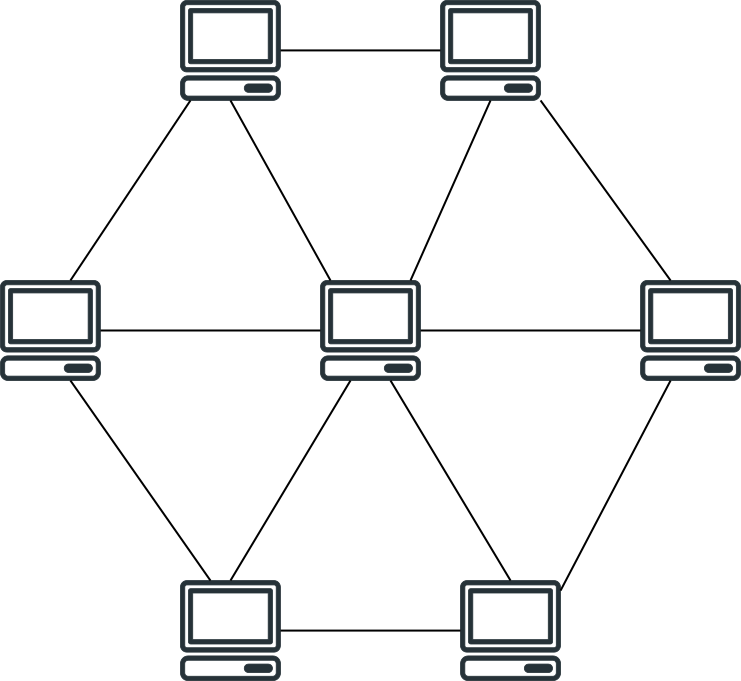
The architecture of the P2P system is shown in the figure above. By eliminating the central server, the P2P system is much more stable: the failure of a few nodes hardly affects the whole service; the nodes are mostly provided by users, so that “the wildfire can’t burn out, the wind can blow again”. Even if someone tries to break the system, it will not be able to hit the whole system effectively.
2.2 Plain P2P networks
One of the most important problems that P2P networks need to solve is how to know which node a user is requesting resources from. In the first generation of P2P networks, a central server was set up to manage the location of resources. When a user wants to post a resource, he needs to tell the central server about the resource he is posting and his node information; when other users request a resource, they need to request the central server to get the node information of the resource publisher first, and then request the resource from the resource publisher.
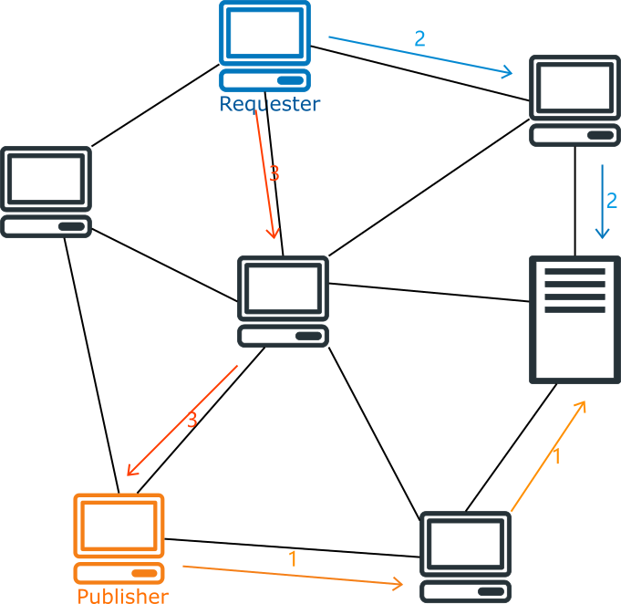
The advantage of this P2P network is its high efficiency, as it only needs to request the central server once to publish or obtain resources. However, its disadvantage is also obvious: the central server is the most vulnerable part of the network system, it needs to store information about all resources and handle requests from all nodes; once the central server fails, the whole network becomes unusable.
Another early P2P network adopts a different strategy, it does not have a central server; when a user requests a resource, it requests all its neighboring nodes, which in turn request their respective neighboring nodes, and uses some policies to prevent duplicate requests until it finds the node with the resource. In other words, this is a kind of Flooding Search.
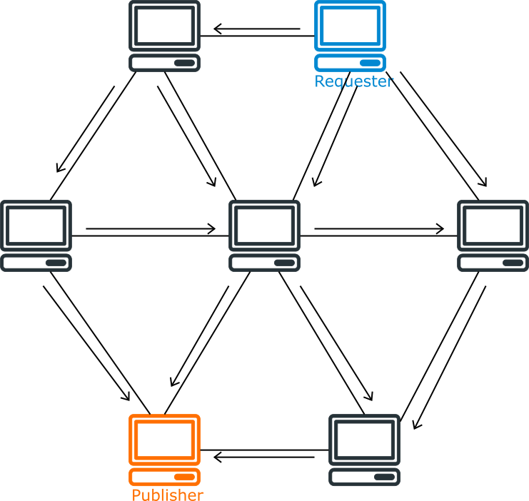
This P2P network is much more stable without the central server. However, it is too slow. One lookup may generate a large number of requests, and a large number of nodes may be involved. Once there are too many nodes in the system, the performance becomes very poor.
2.3 Distributed Hash Tables
To solve these problems, distributed hash tables are created. In a distributed hash table with $n$ nodes, each node only needs to store $\mathrm{O}(\log n)$ other nodes, and only $\mathrm{O}(\log n)$ nodes need to be requested when searching for resources, and no central server is needed, it is a completely self-organizing system. There are many algorithms for implementing distributed hash tables, two of which are described in detail in Sections 3 and 4. Here we will first look at the ideas they share.
Address Management
First, in a distributed hash table, each node and resource has a unique identifier, which is usually a 160-bit integer. For convenience, we call the unique identifier of a node ID and the unique identifier of a resource Key. We can hash the IP address of a node with SHA-1 algorithm to get the ID of the node; similarly, we can hash a resource file with SHA-1 algorithm to get the Key of the resource.
Once the ID and Key are defined, the resources can be published and stored. Each node is responsible for a specific range of keys, the rules of which depend on the specific algorithm. For example, in the Chord algorithm, each Key is always the responsibility of the first node with an ID greater than or equal to it. When a resource is published, the key of the resource file is first calculated by a hashing algorithm, and then the node responsible for this key is contacted and the resource is stored on this node. When someone requests the resource, contact the node responsible for this key and retrieve the resource.
There are two ways to publish and request resources, one is to transfer the file directly to the responsible node, which stores the file resources, and then the node transfers the file to the requestor when the resources are requested. The other approach is for the publisher to try to store the resource itself, transferring the address of the node where the file is located to the responsible node when publishing the file, with the responsible node storing only one address; when requesting the resource, it contacts the responsible node to get the address of the resource file, and then retrieves the resource. Both approaches have their advantages and disadvantages. The advantage of the former is that the publisher of the resource does not have to be online for the requestor to get the resource; the disadvantage is that if the file is too large, it incurs large transmission and storage costs. The latter approach has the advantage of lower transfer and storage costs, but the publisher of the resource, or the node where the resource file is located, must be online at all times.
Routing Algorithm
Above we have briefly described the address system, and how to publish and retrieve resources. But now there is a big problem: how to find the node responsible for a particular key? This is where the routing algorithm comes in. Different distributed hash table implementations have different routing algorithms, but the idea is the same.
First of all, each node will be contacted by several other nodes (IP addresses, ports), called routing tables. In general a distributed hash table with $n$ nodes, the length of a node’s routing table is $\mathrm{O}(\log{n})$. Each node constructs a routing table according to specific rules, and eventually all nodes form a network. A message from a node will approach the target node along the network according to a specific routing rule, and finally reach the target node. In a distributed hash table with $n$ nodes, this process is usually forwarded $\mathrm{O}(\log{n})$ times.
Self-organization
The nodes in a distributed hash table are composed of individual users who join, leave, or fail at any time; and there is no central server for the distributed hash table, which means that the system is completely unmanaged. This means that assigning addresses, constructing routing tables, joining nodes, leaving nodes, and excluding failed nodes all rely on self-organizing policies.
To publish or acquire resources, a node must first join. There are usually several steps for a node to join. First, a new node needs to contact any existing node in the distributed hash table through some external mechanism; then the new node constructs its own routing table by requesting this existing node and updates the routing tables of other nodes that need to be connected to it; finally the node needs to retrieve the resources it is responsible for.
In addition, we must consider node failures to be a frequent occurrence and must be able to handle them properly. For example, if a node fails during the routing process, there are other nodes that can replace it to complete the routing operation; the nodes in the routing table are periodically checked for validity; resources are repeatedly stored on multiple nodes to counteract node failures, etc. In addition, nodes in the distributed hash table are joined voluntarily and can leave voluntarily. Node departure is handled similarly to node failure, but there are additional operations that can be done, such as immediately updating the routing table of other nodes, dumping their resources to other nodes, etc.
3. Chord Algorithm
The previous section briefly introduced P2P networks and distributed hash tables, and now we discuss a concrete implementation of it. There are many implementations of distributed hash tables, but Ion Stoica and Robert Morris et al. proposed the Chord algorithm in a 2001 paper, which is given in the references at the end of the paper. The Chord algorithm is relatively simple and beautiful, and we present it here first.
3.1 Address Management
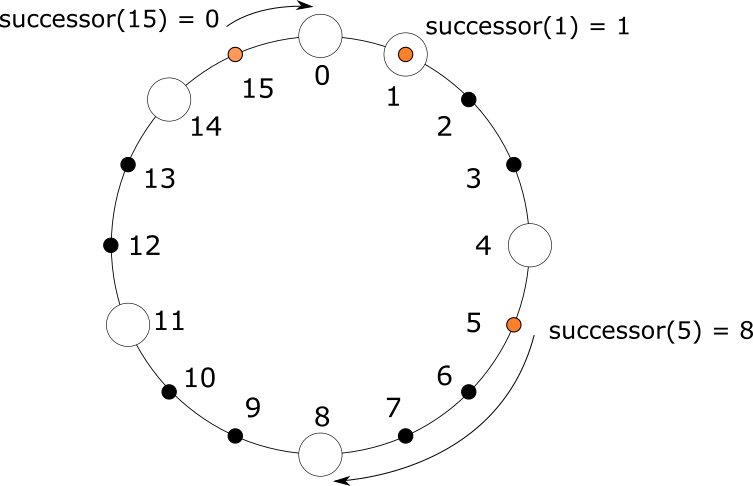
As described in Section 2.3, Chord uses an m-bit integer as a unique identifier for nodes and resources. This means that the identifier is an integer in the range $0$ to $2^m-1$. Chord arranges all IDs in a ring, clockwise from smallest to largest, and end to end. For convenience, we say that each ID is preceded by its counterclockwise ID and followed by its clockwise ID. Each node finds its position in this ring; for a resource with Key k, it will always be the responsibility of the first node whose ID is preceded by or equal to k. We call the node responsible for k. We call the node responsible for k a successor of k, denoted $successor(k)$. For example, as shown in the figure below, in a Chord ring with m = 4, there are six nodes with IDs 0, 1, 4, 8, 11, and 14. The resource with Key 1 is taken care of by the node with ID 1, the resource with Key 5 is taken care of by the node with ID 8, and the resource with Key 15 is taken care of by the node with ID 0. That is, we have $successor(1)=1$, $successor(5)=8$, and $successor(15)=0$.
3.2 Routing Algorithm
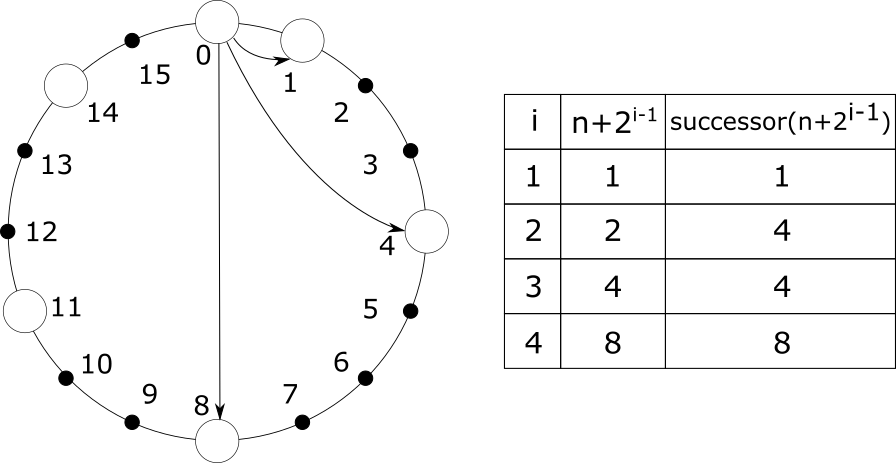
In the Chord algorithm, each node keeps a routing table of length m, storing information about up to m other nodes, which allows us to contact them. Suppose a node has ID n (hereafter node n), then the i-th node in its routing table should be the first node whose ID is first or equal to $n+2^{i-1}$, i.e., $successor(n+2^{i-1})$, where $1 \leqslant i \leqslant m$. We denote the i-th node in the routing table of n as $n.finger[i]$. Obviously, the first node in the routing table is the node next to n in the clockwise direction, which we usually call the successor of n, and is denoted as $n.successor$.
With this routing table, we can address nodes quickly. Suppose a node n needs to find the node where the resource with Key k is located, i.e., it looks for $successor(k)$. It first determines whether k falls in the interval $(n, n.successor]$; if it does, then this Key is the responsibility of its successor. Otherwise, n traverses its own routing table from backward to forward until it finds a node with an ID later than k, and then passes k to that node to perform the above search until it finds it.
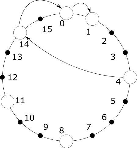
The above figure shows the process of finding node 1 from node 4. Node 4 has nodes 8, 11, and 14 in its routing table. It first finds the first node after 1 in its routing table as 14 from backward to forward, and then asks 14 to help find 1. Node 14 has nodes 0, 4, and 8 in its routing table; similarly, 14 asks node 0 to help find 1. Finally, node 0 finds its successor as node 1.
As we can see, the whole process of finding is to approach the target node step by step. The further away from the target node, the longer the jump distance; the closer to the target node, the shorter and more accurate the jump distance. If the whole system has N nodes, the number of jumps performed in the search is $\mathrm{O}(\log N)$.
3.3 Self-organization
Node Joining
It is not hard for a node to join Chord. As mentioned in the previous section, any node in the Chord system can find its successor $successor(k)$ for any key k. First, the new node $n$ uses some algorithm to generate its own ID, and then it needs to contact any node $n’$ in the system and ask it to help find $successor(n)$. Obviously, $successor(n)$ is the successor of n and the first node in its routing table. It then asks $n’$ to help it find $successor(n + 2^1)$, $successor(n + 2^2)$, etc., until it finishes building its own routing table.
After building its own routing table, n is basically added to Chord. But it is not enough, because at this point the other nodes do not know it exists. After n joins, some nodes still have pointers to n’s successors in their routing tables. This is the time to remind these nodes to update their routing tables. Which nodes need to update their routing tables? We simply reverse the operation: for all $1 \leqslant i \leqslant m$, find the first node that is after $n - 2^{i-1}$. This is the same as finding a successor, and will not be repeated.
Finally, the new node n also needs to retrieve all the resources it is responsible for. n just needs to contact its successor to retrieve all the resources owned by its successor whose Key is later than or equal to n.
Handling Concurrency Issues
Consider multiple nodes joining Chord at the same time. If the above method is used, it may lead to inaccurate routing tables. For this reason, we cannot update the routing table of all nodes at once when a new node is added. It is very important for the Chord algorithm to ensure that each node’s successors are accurate. To ensure this, we want each node to be able to communicate with its successor nodes in both directions, checking each other. Therefore, we add a property $n.predecessor$ to each node that points to its predecessor node. Then, we have each node periodically perform an operation called $stabilize$. In the $stabilize$ operation, each node $n$ asks its successor $s$ for $s$’s predecessor node $x$. Then $n$ checks whether $x$ is more suitable as its successor, and if so, $n$ updates its own successor to $x$. At the same time $n$ tells its successor $s$ about its existence, and $s$ checks whether $n$ is better suited to be its predecessor, and if so, $s$ updates its predecessor to $n$. This operation is simple enough to ensure the accuracy of the Chord ring.
When a new node $n$ joins the Chord, it first contacts the existing node $n’$ to get $n.successor$. $n$ does nothing but set up its successor; at this point $n$ has not yet joined the Chord ring. This is done after $stabilize$ is executed: when $n$ executes $stabilize$, it notifies its successor to update its predecessor to $n$; when $n$’s real predecessor $p$ executes $stabilize$, it fixes its successor to $n$ and notifies $n$ to set its predecessor to $p$. Thus $n$ is added to the Chord ring. This is also true for multiple nodes joining at the same time.
In addition, each node $n$ periodically repairs its own routing table to ensure that it points to the correct node. This is done by randomly picking the $i$th node in the routing table, finding and updating $n.finger[i]$ to $successor(n+2^{i-1})$. Since the successor node of $n$ is always correct, this lookup operation is always valid.
Node Failure and Departure
When a node fails, it will inevitably cause a node’s successor to fail. The accuracy of the successor node is crucial to the Chord, as its failure means that the Chord ring is broken, which may cause the lookup to fail and the $stabilize$ operation to fail. To solve this problem, a node usually maintains multiple successor nodes, forming a successor list, which is usually of length m. In this way, when a node’s successor node fails, it searches for the next replacement node in the successor list. In addition, the failure of a node implies the loss of resources on that node, so a resource is repeatedly stored on several successors of n, in addition to the node n responsible for it.
The handling of a node leaving is similar to node failure, except that a node can perform some additional actions when it leaves, such as notifying its surrounding nodes to immediately perform the $stabilize$ operation, transferring resources to its successors, etc.
4. Kademlia’s Algorithm
Petar Maymounkov and David Mazières proposed the Kademlia algorithm in a paper in 2002, which is given in the references at the end of the paper. The Kademlia algorithm is more fault-tolerant than the Chord algorithm, more efficient than Chord, and more clever and reasonable.
4.1 Address management
Kademlia also uses m-bit integers as unique identifiers for nodes and resources. Unlike the “interval responsibility” system in Chord, resources in Kademlia are the responsibility of the node closest to it. For fault-tolerance reasons, each resource is usually responsible for the k nodes closest to it, where k is a constant, usually taken to make it unlikely that any k nodes in the system will fail simultaneously within an hour, e.g., k = 20. Interestingly, the “distance” here is not a numerical difference, but is derived by a heterogeneous operation. In Kademlia, each node can be considered as a leaf node in a binary tree of height m + 1. The ID is binary expanded, starting from the highest bit, going from the root node to the left and 0 to the right, until it reaches the leaf node. This is shown in the figure below.

The cleverness of Kademlia is to define the distance between two IDs $x$ and $y$ as $x \oplus y$. If the high bits of the two IDs are different and the low bits are the same, the result of their dissimilarity is larger; if the high bits are the same and the low bits are different, the result of the dissimilarity is smaller. This is consistent with the distribution of leaf positions in a binary tree: if two nodes share fewer ancestors (with different highs), they are far apart; conversely, if they share more ancestors (with the same highs), they are close together. The above figure shows the distance between some nodes, you can feel it.
Another important property of heteroskedasticity is that the inverse of heteroskedasticity is still heteroskedasticity. That is, if we have $x \oplus y = d$ then $x \oplus d = y$. This means that for each node, given a distance $d$, there is at most one node with a distance $d$ from it. In this way the topology of Kademlia is unidirectional. Unidirectionality ensures that all lookups for the same Key converge along the same path, no matter which node the lookup starts from.
4.2 Routing algorithm
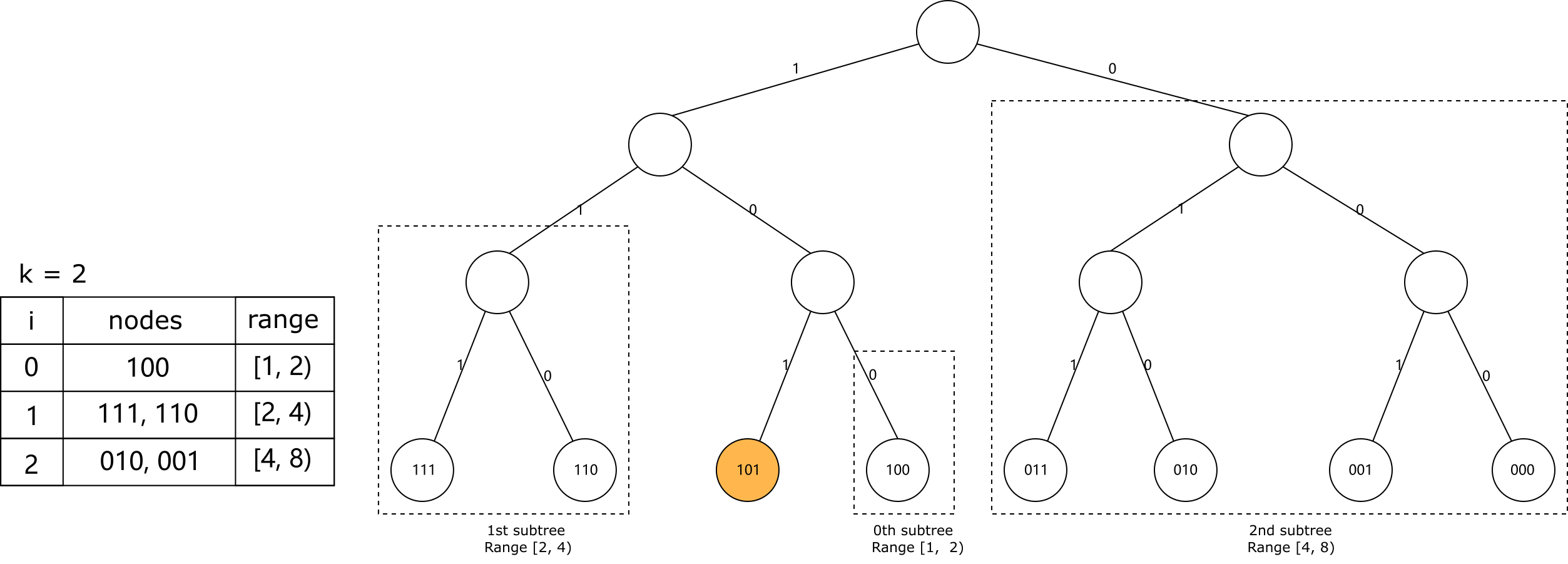
For any given node, we divide the binary tree from the root node into a series of subtrees that do not contain that node. The highest subtree consists of half of the binary tree that does not contain that node, the next subtree consists of the remaining half of the tree that does not contain that node, and so on. If the height of this binary tree is m + 1, we end up with m subtrees. Then we take any k nodes in each subtree, forming m k-buckets, which are the routing tables of Kademlia nodes. We define the node obtained in the smallest subtree as the 0th k-bucket, the node obtained in the next smallest subtree as the 1st k-bucket, and so on. It is easy to see that for each $0 \leqslant i < m$, the distance between the node in the $i$th k-bucket and the current node is always within the interval $[2^i, 2^{i+1})$. The following figure shows the k-buckets of node 101 for m = 3 and k = 2.
Each node in Kademlia has a base operation, called the FIND_NODE operation. FIND_NODE takes a Key as an argument and returns the k nearest nodes to this Key that the current node knows. Based on the k-buckets, it is easy to find the k nearest nodes: first find the distance $d$ between the Key and the current node; as mentioned above, the distance between the node in the $i$th k-bucket and the current node is always within the interval $[2^i, 2^{i+1})$, and these intervals do not overlap each other, so obviously the node in the k-bucket where $d$ falls is the nearest node to the Key. node. If there are less than k nodes in this k-bucket, the node is added to the next k-bucket, and if not, the node is added to the next k-bucket. If the sum of all k buckets of the node is less than k nodes, it returns all the nodes it knows.
With the FIND_NODE operation, we can define the most important procedure in Kademlia, node lookup. What a node lookup does is, given a Key, find the k nodes closest to it in the entire system. This is a recursive process: first the initial node calls its own FIND_NODE and finds the k nodes it knows are closest to the Key. Next we take the $\alpha$ nearest nodes among these k nodes and ask them to perform FIND_NODE for the Key. Here $\alpha$ is also a constant, which is used to request efficiency at the same time, e.g. $\alpha = 3$.
In the recursive process that follows, the initial node takes the nearest $\alpha$ nodes that have not been requested after the previous request and requests them to perform FIND_NODE for the Key, and so on. Each time it is executed, the node returned is closer to the target. If the node returned by a request is not closer to the target Key than the node returned by the last request, request FIND_NODE from all nodes that have not been requested. If no closer node can be fetched, the process terminates. At this point we take the k nodes closest to the Key, which is the result of the node lookup.
Most of Kademlia’s operations are based on node lookups. When publishing a resource, we simply perform a node lookup for the resource’s Key, get the k nodes closest to the resource, and store the resource on those nodes.
The same is true for fetching a resource, where a node lookup is performed for the target resource’s Key, except that the lookup stops once it encounters a node that owns the target resource. In addition, once a node succeeds in its lookup, it caches the resource on the node closest to it. Since Kademlia’s topology is unidirectional, other nodes farther away from the target resource than itself are likely to pass through the cached node during lookup, which improves lookup efficiency by terminating the lookup earlier.
4.3 Self-organization
k bucket maintenance
All k-buckets follow the Least Recently Used (LRU) elimination method. The least recently active nodes are ranked at the head of the k-bucket, and the most recently active nodes are ranked at the end of the k-bucket. When a Kademlia node receives any message (request or response) from another node, it tries to update the corresponding k-bucket. If the node is in the recipient’s corresponding k-bucket, the recipient moves it to the end of the k-bucket. If the node is not in the corresponding k-bucket and there are less than k nodes in the k-bucket, then the receiver inserts the node directly into the tail of the k-bucket. If the corresponding k-bucket is full, the receiver tries to ping the least active node in the k-bucket. If the least active node fails, it removes it and inserts the new node at the end of the k-bucket; otherwise, it moves the least active node to the end of the k-bucket and discards the new node.
By this mechanism, the k-bucket can be refreshed while communicating. In order to prevent some range of keys from not being easily found, each node manually refreshes the k-bucket that has not performed a lookup in the previous hour. This is done by selecting a random key in this k-bucket and performing a node lookup.
Node Joining
For a new node $n$ to join Kademlia, it first generates its own ID using some algorithm, then it needs to obtain any node $n’$ in the system by some external means and add $n’$ to the appropriate k bucket. Then it performs a node lookup on its own ID. According to the above k-bucket maintenance mechanism, the new node $n$ automatically constructs its own k-bucket during the lookup process and inserts itself into the k-bucket of other suitable nodes without any other operations.
When a node joins, in addition to building a k-bucket, it should also retrieve the resources for which the node is responsible. Kademlia does this by performing a publish operation on the resources owned by all nodes at regular intervals (e.g., one hour); in addition, at regular intervals (e.g., 24 hours) nodes discard resources that have not received a publish message during that time. In this way, new nodes receive the resources they are responsible for, and the resources are always kept in the hands of the k nodes closest to them.
It would be wasteful if all nodes re-posted the resources they have every hour. To optimize this, when a node receives a resource release message, it does not retransmit it in the next hour. This is because when a node receives a resource release, it can assume that k - 1 other nodes have also received the resource release. This ensures that each resource is always re-posted by only one node, as long as the nodes do not re-post resources at the same pace.
Node Failure and Departure
With the above k-bucket maintenance and resource retransmission mechanisms, we do not need to do anything else for node failures and departures. This is the cleverness of the Kademlia algorithm, which is more fault-tolerant than other distributed hash table algorithms.
5. Summary
This article introduced P2P technology and distributed hash tables, as well as two distributed hash table algorithms, basically introducing their principles and implementation mechanisms. The text is also a summary of the author’s study of these two papers, and for the sake of space and effort, some implementation details, theoretical and experimental support behind the strategy, proof of the algorithm, etc. are not elaborated. It is recommended that students who want to learn more read the reference material. Building a P2P architecture is a challenging task, and I think it is useful to understand and learn P2P technologies for server architecture even if you are not engaged in P2P development.