Big Data Foundation: Google GFS

Introduction to the GFS system

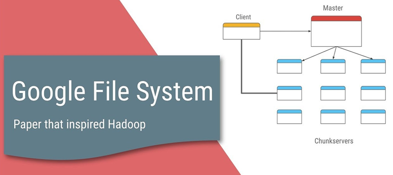
Google File System (abbreviated as GFS or GoogleFS), a proprietary distributed file system developed by Google Inc.

It differs from traditional file systems in that it is.

• Distributed - provides a high degree of horizontal scalability
• Networked using a large number of inexpensive common machines - allows for single machine failure
• No Random Write - does not allow arbitrary changes to existing files

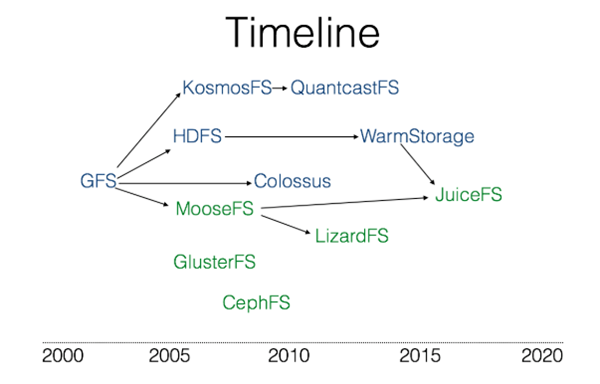
Google did not release the software part of the system as open source software. Instead, it published a paper on “The Google File System”. The HDFS in Hadoop is built with reference to Google’s paper. The following diagram shows a branch of the file system based on the GFS file system.

The Google File System Chinese Translation

Abstract

We designed and implemented the Google GFS file system, a scalable distributed file system for large-scale data-intensive applications. gfs runs on inexpensive and common hardware devices, but it still provides disaster redundancy and high performance for a large number of clients.

While the design goals of GFS have much in common with many traditional distributed file systems, our design is based on our analysis of our own application load profile and technical environment, both now and in the future, and GFS is significantly different from earlier distributed file system visions. So we revisited the traditional file system design trade-off choices and derived a completely different design idea.

GFS fully meets our storage needs and has been widely deployed as a storage platform within Google, storing data generated and processed by our services, as well as for research and development work that requires large data sets. By far the largest cluster leverages thousands of hard drives on thousands of machines, providing hundreds of terabytes of storage space while serving hundreds of clients.

In this thesis, we show extensions to the file system interface that can support distributed applications, discuss many aspects of our design, and finally list small-scale performance tests as well as performance-related data from real production systems.

1. Introduction

In order to meet Google’s rapidly growing data processing needs, we designed and implemented the Google File System (GFS), which shares many of the same design goals as traditional distributed file systems, such as performance, scalability, reliability, and availability. However, our design is also influenced by our observations of our own application load profile and technical environment, both now and in the future, and GFS is significantly different from the assumptions of earlier file systems. So we revisited the design tradeoffs of the traditional file system and derived a completely different design philosophy.

• First, component failure is considered a constant event, not an accident. gfs consists of hundreds or even thousands of storage machines assembled from ordinary, inexpensive devices and accessed by a significant number of clients at the same time. the number and quality of gfs components leads to the fact that it is possible for some components to fail to work at any given time, and for some components to fail to recover from their current state of failure. We have encountered a variety of problems, such as application bugs, operating system bugs, human error, and even problems caused by hard disk, memory, connector, network, and power supply failures. Therefore, mechanisms for continuous monitoring, error detection, disaster redundancy, and automatic recovery must be integrated into GFS.
• Second, our files are huge by common standards. Files of several gigabytes are very common. Each file typically contains many application objects, such as web documents. When we often have to deal with rapidly growing, terabyte-sized data sets consisting of hundreds of millions of objects, it would be very unwise to manage hundreds of millions of small KB-sized files, even though some file systems support such a management approach. Therefore, design assumptions and parameters, such as I/O operations and Block sizes, need to be reconsidered.
• Third, the vast majority of files are modified by appending data to the end of the file, rather than overwriting the original data. Random writes to the file are virtually non-existent in practice. Once the write is complete, the only operations on the file are reads, usually sequentially. Large amounts of data fit these characteristics, such as: very large data sets scanned by data analysis programs; continuous streams of data generated by running applications; archived data; and intermediate data generated by one machine and processed by another machine, which may be processed simultaneously or later. For this access model for massive files, it does not make sense for the client to cache blocks of data, and the appending of data is a major consideration for performance optimization and atomicity assurance.
• Fourth, the co-design of application and file system APIs improves the flexibility of the overall system. For example, we relaxed the requirements of the GFS consistency model, which eases the demanding requirements of the file system on the application and greatly simplifies the design of GFS. We introduce atomic record append operations, thus ensuring that multiple clients can perform append operations simultaneously without requiring additional synchronization operations to ensure data consistency. Details of these issues are discussed in more detail later in this paper.

Google has deployed several GFS clusters for different applications. The largest cluster has over 1000 storage nodes and over 300TB of hard disk space, which is accessed frequently and continuously by hundreds of clients on different machines.

2. Design Overview

2.1 Design Expectations

In designing a file system that meets our needs, our design goals present both opportunities and challenges. We have previously mentioned some of the key points to focus on, and here we expand on the details of the design’s intended goals.

• The system consists of many inexpensive, common components, and component failure is a constant. The system must continuously monitor its own state, it must treat component failure as a constant, and be able to quickly detect, redundantly and recover from failed components.
• The system stores a certain number of large files. We expect to have several million files, with file sizes typically at or above 100MB. Files several gigabytes in size are also common and have to be able to be managed efficiently. The system must also support small files, but does not need to be optimized specifically for small files.
• The system workload consists of two main types of read operations: large scale streaming reads and small scale random reads. Large-scale streaming reads typically read hundreds of kilobytes of data at a time, and more commonly read 1MB or more at a time. A sequential operation from the same client usually reads a contiguous region of the same file. Small random reads typically read a few KB of data at a random location in the file. If the application is very concerned about performance, it is common practice to combine and sort small random read operations and then read them in sequential batches, thus avoiding the need to move the read location back and forth in the file.
• The system workload also includes many large scale, sequential, data append style write operations. Typically, the size of each write is similar to that of a mass read. Once data has been written, the file is rarely modified. The system supports small-scale, random-position write operations, but they may not be efficient.
• The system must be efficient, with well-defined behavior, to achieve the semantics of multiple clients appending data to the same file in parallel. Our files are often used in “producer-consumer” queues, or other multiplexed file merging operations. There are typically hundreds of producers, each running on a single machine, appending to a single file at the same time. Atomic multiple append data operations with minimal synchronization overhead are essential. The file can be read later, or the consumer can read the file at the same time as the append operation.
• Stable network bandwidth for high performance is far more important than low latency. The vast majority of our target programs require the ability to process data at high rates and in large batches, and very few have strict response time requirements for a single read or write operation.

2.2 Interfaces

GFS provides a set of API interface functions similar to a traditional file system, although not strictly implemented in the form of a standard API such as POSIX. Files are organized as hierarchical directories, identified by pathnames. We support common operations such as creating new files, deleting files, opening files, closing files, reading and writing files.

In addition, GFS provides snapshot and record append operations. Snapshots create a copy of a file or directory tree at a very low cost. Record Append allows multiple clients to simultaneously append data to a file while ensuring that each client’s append operation is atomic. This is useful for implementing multiplexed result merges, and “producer-consumer” queues, where multiple clients can append data to a file simultaneously without additional synchronization locking. We have found these types of files to be very important for building large distributed applications. Snapshot and record append operations are discussed in sections 3.4 and 3.3, respectively.

2.3 Architecture

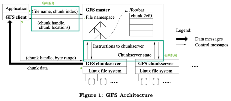
A GFS cluster contains a single Master node, multiple Chunk servers, and is accessed by multiple clients at the same time, as shown in Figure 1. All these machines are usually ordinary Linux machines running user-level service processes. We can easily put both Chunk servers and clients on the same machine, provided that the machine resources allow it and we can accept the risk of reduced stability from unreliable application code.

When a chunk is created, the Master server assigns each chunk an unchanging, globally unique 64-bit chunk identifier. The Chunk server stores the Chunk as a linux file on the local hard disk and reads and writes the chunk data according to the specified Chunk identifier and byte range. For reliability reasons, each chunk is replicated to multiple chunk servers. By default, we use 3 storage replication nodes, but users can set different replication levels for different file namespaces.

The Master node manages all file system metadata. This metadata includes namespaces, access control information, file and Chunk mapping information, and current Chunk location information. master nodes also manage system-wide activities such as Chunk lease management, orphan Chunk reclamation, and Chunk migration between Chunk servers. master nodes use heartbeat information The Master node communicates with each Chunk server periodically, sending commands to each Chunk server and receiving status information from the Chunk servers.

The GFS client code is linked to the client program as a library. The client code implements the GFS file system API functions, application communication with the Master node and Chunk servers, and read and write operations on data. The communication between the client and the Master node only gets metadata, all data operations are performed by the client directly with the Chunk server. We do not provide the functionality of the POSIX standard API, so GFS API calls do not need to go down to the Linux vnode level.

Neither the client nor the Chunk server needs to cache file data. There is little use for client-side caching of data, since most programs either read a huge file as a stream or have a working set that is simply too large to be cached. Not having to think about cache-related issues also simplifies the design and implementation of the client and the system as a whole. (However, the client does cache metadata.) The reason the Chunk server does not need to cache file data is that Chunk is stored as a local file, and the Linux OS file system cache caches frequently accessed data in memory.

2.4 Single Master Node

The single Master node strategy greatly simplifies our design. A single Master node can pinpoint the location of Chunk and make replication decisions with global information. In addition, we must reduce the number of reads and writes to the Master node to avoid the Master node becoming the bottleneck of the system. The client does not read or write file data through the Master node. Instead, the client asks the Master node for the Chunk server it should contact. The client caches this metadata information for a period of time, and subsequent operations will be performed directly with the Chunk server for data read and write operations.

Let’s use Figure 1 to explain the flow of a simple read. First, the client takes the file name and the byte offset specified by the program and converts it into the Chunk index of the file based on a fixed Chunk size. Then, it sends the file name and Chunk index to the Master node, which sends the corresponding Chunk identifier and the location information of the replica back to the client. The client uses the file name and Chunk index as the key to cache this information.

The client then sends a request to one of the replicas, usually choosing the closest one. The request message contains the Chunk’s identity and byte range. For subsequent reads of this chunk, the client does not need to communicate with the master node unless the cached metadata information is out of date or the file is reopened. In practice, clients often query multiple Chunks in a single request, and the Master node’s response may also contain information about the Chunk that immediately follows the requested Chunk. In practice, this extra information avoids, at no cost, several possible future communications between the client and the Master node.

2.5 Chunk Size

The size of Chunk is one of the key design parameters. We chose 64MB, a size much larger than the block size of a typical file system. a copy of each Chunk is stored on the Chunk server as a normal Linux file and is only expanded when needed. The inert space allocation policy avoids wasted space due to internal fragmentation, which is perhaps the most controversial point about choosing such a large Chunk size.

Choosing a larger Chunk size has several important advantages. First, it reduces the need for clients to communicate with the Master node, because only one communication with the Mater node is needed to obtain the Chunk location information, and then multiple read and write operations can be performed on the same Chunk. This approach has a significant effect on reducing our workload, since our application usually reads and writes large files continuously. Even for small random reads, there is a clear benefit to using a larger Chunk size, as the client can easily cache all the Chunk location information for a multi-terabyte working data set. Second, with a larger Chunk size, the client can perform multiple operations on a chunk, which reduces the network load by maintaining a longer TCP connection to the Chunk server. Third, choosing a larger Chunk size reduces the amount of metadata that the Master node needs to store. This allows us to keep all metadata in memory, and we will discuss the additional benefits of having all metadata in memory in Section 2.6.1.

On the other hand, using a larger Chunk size has its drawbacks, even in conjunction with inert space allocation. Small files contain fewer Chunks, or even only one Chunk, and when there are many clients making multiple accesses to the same small file, the Chunk server storing these Chunks becomes a hotspot. In practice, hotspots are not a major problem because our application usually reads large files containing multiple Chunks in succession.

However, the hotspot problem arose when we first used GFS for a batch queuing system: an executable file was saved as a single-chunk file on GFS, and then the executable was started on hundreds of machines at the same time. The several Chunk servers where the executable is stored are accessed by hundreds of concurrent client requests resulting in a local overload of the system. We solved this problem by using larger replication parameters to hold the executable and by staggering the start time of the batch queue system programs. A possible long-term solution is to allow clients to read data from other clients in such cases.

2.6 Metadata

The Master server stores 3 main types of metadata, including: file and Chunk namespaces, file and Chunk correspondences, and where each Chunk copy is stored. All metadata is stored in the memory of the Master server. The first two types of metadata (namespaces, file-chunk relationships) are also recorded in the OS syslog file as change logs, which are stored locally on disk and copied to other remote Master servers. By keeping the changelog, we can easily and reliably update the status of the Master server without the risk of inconsistent data due to a crash of the Master server. The Master server does not persist Chunk location information.

2.6.1 In-memory data structure

Because the metadata is stored in memory, the Master server is very fast to operate. Moreover, the Master server can scan all the state information it keeps in the background in a simple and efficient periodic manner. These periodic state scans are also used for Chunk garbage collection, data replication in case of Chunk server failure, load balancing across Chunk servers through Chunk migration, and disk usage statistics, etc. These behaviors are discussed in depth in sections 4.3 and 4.4.

There is a potential problem with keeping all metadata in memory: the number of Chunks and the capacity of the entire system are limited by the amount of memory available to the Master server. In practice, however, this is not a serious problem; the Master server requires less than 64 bytes of metadata to manage a 64MB Chunk, and since most files contain multiple Chunks, most Chunks are full, except for the last Chunk of the file, which is partially populated. Similarly, the data size of each file in the namespace is usually less than 64 bytes, because the saved filenames are compressed using a prefix compression algorithm.

Even when larger file systems need to be supported, the cost of adding additional memory to the Master server is minimal, and by adding a limited amount of cost, we are able to keep all of the metadata in memory, enhancing the simplicity, reliability, performance, and flexibility of the system.

2.6.2 Chunk Location Information

The Master server does not keep information about which Chunk server holds a copy of a given Chunk persistently; the Master server only polls the Chunk server for this information at boot time. The Master server can ensure that the information it holds is always up-to-date because it controls the allocation of all Chunk locations and monitors the state of the Chunk server with periodic heartbeat messages.

Initially, we tried to keep the Chunk location information persistent on the Master server, but later we found it simpler to poll the Chunk server at startup and then poll it periodically for updates. This design simplifies the problem of synchronizing Master and Chunk server data when Chunk servers join, leave, rename, fail, and restart the cluster. In a cluster with hundreds of servers, such events can happen frequently.

This design decision can be understood from another perspective: only the Chunk server can ultimately determine whether a Chunk is on its hard drive. We never considered maintaining a global view of this information on the Master server, because a Chunk server error could cause a Chunk to automatically disappear (e.g., a drive is corrupted or inaccessible), or the operator could rename a Chunk server.

2.6.3 Operation Log

The operation log contains a history of key metadata changes. This is very important to GFS. This is not only because the operation log is the only persistent storage record for metadata; it also serves as a logical time baseline for determining the order of synchronization operations. Files and Chunk, along with their versions (refer to section 4.5), are uniquely and permanently identified by the logical time they were created.

The operation logs are very important and we must ensure the integrity of the log files and that the logs are visible to the client only after changes to the metadata have been persisted. Otherwise, even if there is nothing wrong with Chunk itself, we may still lose the entire file system or lose the client’s recent operations. The Master server collects multiple log records and processes them in bulk to reduce the impact of writing to disk and replication on overall system performance.

The Master server restores the file system to its most recent state by replaying the operation logs during disaster recovery. To shorten the Master boot time, we must keep the logs small enough for the Master server to do a checkpoint on the system state when the logs grow to a certain size, writing all the state data to a checkpoint file. Checkpoint files are stored in a compressed B-tree structure that can be mapped directly to memory without additional parsing when used for namespace queries. This greatly increases the speed of recovery and enhances availability.

Since it takes time to create a Checkpoint file, the internal state of the Master server is organized in a format that ensures that the Checkpoint process does not block ongoing modification operations. the Master server uses separate threads to switch to the new log file and create the new Checkpoint file. The new Checkpoint file includes all changes made before the switch. For a cluster containing millions of files, it takes about one minute to create a Checkpoint file. Once created, the Checkpoint file is written to local and remote hard drives.

Only the latest Checkpoint file and subsequent log files are required for Master Server recovery. Old Checkpoint files and log files can be deleted, but in case of a catastrophic failure, we usually keep more historical files. checkpoint failures do not have any impact on correctness because the recovery function’s code detects and skips Checkpoint files that are not completed.

2.7 Consistency Model

GFS supports a loose consistency model that is well suited to support our highly distributed applications, while maintaining the advantage of being relatively simple and easy to implement. In this section we discuss the mechanisms that guarantee the consistency of GFS and what it means for applications. We also focus on describing how GFS manages these consistency assurance mechanisms, but the details of the implementation are discussed elsewhere in this thesis.

2.7.1 GFS Consistency Assurance Mechanisms

Modifications to the file namespace (e.g., file creation) are atomic. They are under the control of the Master node only: namespace locks provide guarantees of atomicity and correctness (chapter 4.1); the Master node’s operation log defines the global order of these operations (chapter 2.6.3).

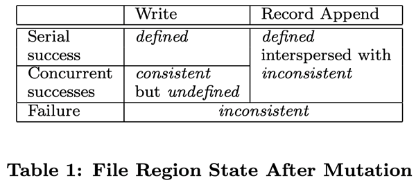
The status of the file region after data modification depends on the type of operation, its success or failure, and whether the modification is synchronized. Table 1 summarizes the results of the various operations. A file region is considered “consistent” if all clients read the same data regardless of which copy they read from; if the region is consistent after modifying the file’s data and the client can see the entire contents of the write operation, then the region is “defined”. When a data modification operation is successfully executed and is not interfered with by other write operations executed at the same time, then the affected region is defined (implicitly consistent): all clients can see the contents of the write. After a parallel modification operation completes successfully, the region is in a consistent, undefined state: all clients see the same data, but cannot read the data written by any of the write operations. Typically, a file region contains a mix of data fragments from multiple modifications. Failed modification operations result in a region being inconsistent (and undefined): different clients will see different data at different times. We will describe later how the application distinguishes between defined and undefined regions, and there is no need for the application to break down the different types of undefined regions.

There are two types of data modification operations: write or record append. A write operation writes data to a file offset location specified by the application. A record append operation appends data atomically to a file at least once, even when multiple modifications are performed in parallel, but the offset location is chosen by the GFS (Chapter 3.3). (In contrast, the offset location for writing the append operation is usually said to be the end of the file.) GFS returns to the client an offset that represents the starting point of the defined region containing the written records. In addition, GFS may insert padding data or duplicate records in the middle of the file. This data occupies a region of the file that is determined to be inconsistent, and is usually much smaller than the user data.

After a series of successful modification operations, GFS ensures that the file region being modified is defined and contains the data written by the last modification operation. (b) use the version number of the Chunk to detect if the replica is invalidated because the Chunk server it is on is down (Chapter 4.5) and the modification operation is missed. The failed replicas are not modified, and the Master server does not return the location information of this Chunk replica to the client. They are reclaimed by the garbage collection system as soon as possible.

Since the Chunk location information is cached by the client, it is possible that the client reads data from a failed copy before the information is refreshed. There is a time window between the timeout of the cache and when the file is next opened, and when the file is opened again it clears the cache of all Chunk location information related to that file. Also, since most of our files are append-only, a failed copy usually returns a prematurely ended Chunk instead of expired data. When a Reader retries and contacts the Master server, it immediately gets the latest Chunk location information.

GFS uses periodic “handshakes” between the Master server and all Chunk servers to find the failed Chunk server, and uses Checksum to verify that the data is not corrupt (Chapter 5.2). Chapter 5.2). As soon as a problem is found, the data is recovered using a valid copy (Chapter 4.3). A Chunk is irreversibly lost only if all copies of the Chunk are lost before GFS detects the error and takes countermeasures. In general the GFS response time (alex: the Master node detects and reacts to the error) is a few minutes. Even in this case, the Chunk is only unavailable, not corrupted: the application receives an explicit error message instead of corrupted data.

2.7.2 Implementation of the program

Applications using GFS can implement this relaxed consistency model using a number of simple techniques that are also used to implement some of the other targeted features, including: appending writes instead of overwrites whenever possible, Checkpoint, self-validating write operations, and self-identifying records.

In practice, all of our applications write to files using data append rather than overwrite as much as possible. In a typical application, the application writes data from start to finish, generating a file. After all the data is written, the application automatically renames the file to a permanent file name or periodically makes a checkpoint to record how much data was successfully written. Checkpoint files can contain program-level checksums; Readers only checks and processes the file regions generated after the last checkpoint, and the state of these file regions must be defined. This approach meets our requirements for consistency and concurrent processing. Writing retroactively is more efficient than writing to random locations and more resilient to application failures. Checkpoint allows Writer to restart in a progressive manner and prevents Reader from processing data that has been successfully written, but has not yet completed from the application’s perspective.

Let’s look at another typical application. Many applications append data to the same file in parallel, for example to perform a merge of results or a producer-consumer queue. The “at least one append” nature of record appending guarantees Writer’s output, and Readers use the following methods to handle occasional padding and duplicate content. Reader can use Checksum to identify and discard additional padding and record fragments. If the application cannot tolerate occasional duplicates (e.g., if they trigger non-idempotent operations), they can be filtered with the record’s unique identifier, which is typically used to name the entity objects processed in the application, such as web documents. These record I/O functions (in addition to rejecting duplicate data) are included in the library shared by our application and are applicable to other file interface implementations within Google. So, the same sequence of records, plus some occasional duplicates, are distributed to the Reader.

3. System Interaction

An important principle that we have used in designing this system is to minimize all operations and Master node interactions. With this design philosophy in mind, we now describe how clients, Master servers, and Chunk servers interact to implement data modification operations, atomic record append operations, and snapshot functionality.

3.1 Lease and Change Order

A change is an operation that changes the contents or metadata of a Chunk, such as a write operation or a record append operation. A change is performed on all copies of the Chunk. The master node creates a lease for one replica of the Chunk, which we call the master Chunk. master Chunk serializes all the change operations of the Chunk. All replicas obey this sequence for modification operations. Therefore, the global order of modification operations is determined first by the order of the lease selected by the master node, and then by the sequence number assigned to the master Chunk in the lease.

The lease mechanism is designed to minimize the administrative burden on the Master node. The initial timeout of the lease is set to 60 seconds. However, whenever a Chunk is modified, the Master Chunk can request a longer lease period, which is usually acknowledged by the Master node and receives a lease extension. These lease extension requests and approvals are usually passed in heartbeat messages attached between the Master node and the Chunk server. Sometimes the Master node tries to cancel the lease early (for example, the Master node wants to cancel a modification operation on a file that has been renamed). Even if the Master node loses contact with the master Chunk, it can still safely sign a new lease with another copy of the Chunk after the old one expires.

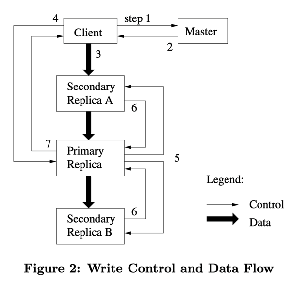
In Figure 2, we show the control flow of the write operation based on the step numbers.

• The client asks the Master node which Chunk server holds the current lease, and the location of the other replicas. If none of the Chunk holds the lease, the Master node selects one of the replicas to establish a lease (this step is not shown on the diagram).
• The Master node returns the identifier of the master Chunk and the locations of the other replicas (also known as secondary replicas, secondaries) to the client. The client caches this data for subsequent operations. The client only needs to re-contact the master node if the primary chunk is not available, or if the master chunk replies with a message indicating that it no longer holds the lease.
• The client pushes the data to all replicas. The client can push data in any order, and the Chunk server receives the data and stores it in its internal LRU cache until it is used or expired and swapped out. Since the network transfer load of the data stream is very high, by separating the data stream from the control stream, we can plan the data stream based on the network topology and improve the system performance without bothering which Chunk server holds the master Chunk.2 This is discussed further in Section 2.
• When all replicas have confirmed the receipt of data, the client sends a write request to the master Chunk server. This request identifies the data that was pushed to all replicas earlier. The master Chunk assigns consecutive sequence numbers to all operations received, which may come from different clients, and the sequence numbers ensure that the operations are executed sequentially. It applies the operations to its own local state in the order of the sequence numbers.
• The primary Chunk passes write requests to all secondary replicas. Each secondary replica performs these operations in the same order according to the sequence number assigned by the primary Chunk.
• All secondary replicas reply to the primary Chunk that they have completed their operations.
• The primary Chunk server replies back to the client. Any errors generated by any replica are returned to the client. In the event of an error, the write operation may execute successfully on the primary Chunk and some secondary copies. (If the operation fails on the primary Chunk, the operation is not assigned a sequence number and is not passed.) The client’s request is recognized as a failure and the region being modified is in an inconsistent state. Our client code handles such errors by repeatedly executing the failed operation. The client makes several attempts from step (3) to step (7) before repeating the execution from the beginning.

If the application writes a large amount of data at once, or if the data spans multiple Chunks, the GFS client code splits them into multiple write operations. These operations all follow the control flow described earlier, but may be interrupted or overwritten by simultaneous operations on other clients. As a result, the tail of a shared file region may contain data fragments from different clients, but nevertheless, because these disaggregated write operations are performed in the same order of completion on all copies, all copies of the Chunk are consistent. This leaves the file region in the consistent, but undefined, state described in Section 2.7.

3.2 Data flow

To improve network efficiency, we took the step of separating the data flow from the control flow. While the control flow goes from the client to the primary Chunk and then to all secondary replicas, the data is pushed sequentially along a carefully selected chain of Chunk servers in a pipelined fashion. Our goal is to leverage the bandwidth of each machine, avoid network bottlenecks and high-latency connections, and minimize the latency of pushing all data.

In order to fully utilize the bandwidth of each machine, data is pushed sequentially along a chain of Chunk servers instead of being pushed in other topological forms (e.g., tree topology). In linear push mode, all of the egress bandwidth of each machine is used to transfer data at the fastest possible speed, rather than dividing bandwidth among multiple recipients.

To avoid network bottlenecks and high-latency links as much as possible (eg, inter-switch is most likely to have similar problems), each machine tries to select the closest machine in the network topology that has not yet received data as the target for pushing data. Suppose the client pushes data from Chunk server S1 to S4. it pushes data to the nearest Chunk server S1. S1 pushes data to S2, because the closest machine between S2 and S4 is S2. similarly, S2 passes data to the closer machine between S3 and S4, and so on and so forth. Our network topology is very simple, and we can calculate the “distance” of nodes by IP address.

Finally, we minimize latency by using a TCP connection-based, pipelined data push method, where the Chunk server receives the data and immediately starts pushing it forward. The pipelined data push helps us a lot because we use a full-duplex switched network. Pushing forward immediately after receiving the data does not slow down the reception speed. In the absence of network congestion, the ideal time to transfer B bytes of data to R copies is B/T + RL, where T is the network throughput and L is the delay in data transfer between the two machines. Typically, we have a network connection speed of 100 Mbps (T), and L will be much less than 1 ms. Thus, 1 MB of data can be distributed in about 80 ms ideally.

3.3 Atomic Record Appending

GFS provides an atomic data appending operation - record appending. In the traditional way of writing, the client program specifies the offset at which the data is to be written. A parallel write operation to the same region is not serial: the region tail may contain multiple data fragments written by different clients. With record appending, the client only needs to specify the data to be written; GFS guarantees that at least one atomic write operation is successfully executed (i.e., a sequential byte stream is written), the written data is appended to the offset specified by GFS, and GFS returns this offset to the client. This is similar to the behavior of multiple concurrent write operations in a Unix OS programming environment for files opened in O_APPEND mode without a race condition.

Record appending is used very frequently in our distributed applications, where there are usually many clients appending writes to the same file in parallel. If we were to write to files in the traditional way, the clients would need additional complex and expensive synchronization mechanisms, such as using a distributed lock manager. In our work, such files are typically used in queue systems with multiple producers/single consumers, or result files that combine data from multiple clients.

Record appending is a modification operation that also follows the control flow described in Section 3.1, except that there is some additional control logic in the main Chunk. The client pushes the data to all copies of the last Chunk of the file, and then sends a request to the master Chunk, which checks whether this record append operation will cause the Chunk to exceed the maximum size (64MB). If the maximum size is exceeded, the master Chunk first fills the current Chunk to the maximum size, then notifies all secondary copies to do the same, and then replies to the client asking it to perform the record append operation again for the next Chunk. (The data size of record appending is strictly limited to 1/4 of the maximum size of the Chunk, so that the number of data fragments is still manageable even in the worst case.) Normally, the appended record does not exceed the maximum size of the Chunk. The primary Chunk appends the data to its own replica, then notifies the secondary replica to write the data in the same location as the primary Chunk, and finally replies to the client that the operation was successful.

If the record append operation fails on any of the replicas, the client needs to re-perform the operation. GFS does not guarantee that all copies of a Chunk are identical at the byte level. It only guarantees that the data as a whole is written at least once atomically. This property can be deduced from a simple observation: if the operation is performed successfully, the data must have been written to all copies of the Chunk at the same offset position. After that, all copies are at least as long as the end of the record, and any subsequent records will be appended to a larger offset address, or to a different Chunk, even if the other Chunk copy is selected as the master Chunk by the Master node. consistent) and vice versa (and therefore undefined). As we discussed in Section 2.7.2, our program can handle inconsistent regions.

3.4 Snapshots

A snapshot operation can make a copy of a file or directory tree (“source”) almost instantaneously and with little disruption to other operations in progress. Our users can use snapshots to quickly create a branch copy of a large data set (often a recursive copy copy), or to back up the current state before doing experimental data operations so that they can easily commit or roll back to the backup state later.

Like AFS, we use the standard copy-on-write technique to implement snapshots. When the master node receives a snapshot request, it first cancels the lease on all chunks of the file it is taking a snapshot of. This measure ensures that subsequent write operations to these chunks must interact with the Master to find the lease holder. This gives the Master node a chance to be the first to create a new copy of the Chunk.

After the lease is cancelled or expired, the Master node logs the operation to its hard disk. The Master node then reflects the changes in this log entry to the state stored in memory by copying the metadata of the source file or directory. The newly created snapshot file and the source file point to the exact same Chunk address.

After the snapshot operation, when the client wants to write data to Chunk C for the first time, it first sends a request to the Master node to query the current lease holder. The Master node notices that the reference count of Chunke C exceeds 1. The Master node does not reply to the client’s request right away, but chooses a new Chunk handle C. After that, the Master node asks each Chunk server that has the current copy of Chunk C to create a new Chunk called C. By creating a new Chunk on the Chunk server where the source Chunk is located, we ensure that the data is replicated locally and not over the network (our hard drives are about 3 times faster than our 100Mb Ethernet). In this respect, the request is handled no differently than any other Chunk: the Master node makes sure that a copy of the new Chunk C` has a lease, and then replies to the client, who gets the reply and can write the Chunk normally, regardless of the fact that it was cloned from an existing Chunk.

4. Master node operations

The Master node performs all namespace operations. In addition, it manages all copies of Chunk in the system: it decides where to store Chunk, creates new Chunk and its copies, coordinates various system activities to ensure that Chunk is fully replicated, load balances among all Chunk servers, and reclaims storage space that is no longer in use. In this section, we discuss the above topics.

4.1 Namespace Management and Locks

Many operations on Master nodes can take a long time: for example, snapshot operations must cancel the leases of all the Chunks involved in the snapshot on the Chunk server. We do not want to delay the operation of other Master nodes while these operations are running. Therefore, we allow multiple operations to run simultaneously, using locks on the region of the namespace to ensure proper execution order.

Unlike many traditional file systems, GFS does not implement a per-directory data structure that lists all files in a directory, nor does it support file or directory linking (i.e., hard or symbolic linking in Unix terms). Logically, the GFS namespace is a lookup table of full path and metadata mapping relationships. Using prefix compression, this table can be efficiently stored in memory. On the tree structure where the namespace is stored, each node (absolute path file name or absolute path directory name) has an associated read/write lock.

Each Master node operation acquires a series of locks before it begins. Typically, if an operation involves /d1/d2/…/dn/leaf, then the operation first obtains read locks for directories /d1, /d1/d2, …, /d1/d2/…/dn, and /d1/d2/…/ dn/leaf for read/write locks. Note that depending on the operation, a leaf can be a file or a directory.

Now, let’s demonstrate how the locking mechanism prevents the creation of the file /home/user/foo when /home/user is snapshot to /save/user. The snapshot operation obtains read locks on /home and /save, and write locks on /home/user and /save/user. The file creation operation obtains read locks on /home and /home/user and write locks on /home/user/foo. These two operations are executed sequentially because the locks on /home/user they are trying to obtain conflict with each other. The file creation operation does not need to obtain a write lock for the parent directory, because there is no “directory” or data structure like inode that prohibits modification. The read lock on the filename is sufficient to prevent the parent directory from being deleted.

The advantage of using this locking scheme is that it supports parallel operations on the same directory. For example, multiple files can be created in the same directory at the same time: each operation acquires a read lock on the directory name and a write lock on the file name. The read lock on the directory name is sufficient to prevent the directory from being deleted, renamed, or snapshotted. The file name write lock serializes file creation operations to ensure that files with the same name are not created multiple times.

Because the namespace may have many nodes, read and write locks are allocated inertly and are removed immediately when no longer in use. Similarly, locks are acquired based on a globally consistent order to avoid deadlocks: first sorted by namespace hierarchy, and within the same hierarchy sorted by dictionary order.

4.2 Location of Copies

A GFS cluster is a highly distributed, multi-layered structure, rather than a flat structure. A typical topology has hundreds of Chunk servers installed in many racks. chunk servers are accessed by hundreds of clients from the same or different racks on a rotating basis. Communication between two machines in different racks may span one or more network switches. In addition, the bandwidth in and out of a rack may be smaller than the sum of all the machines in the rack. Multi-tier distribution architectures present unique challenges in terms of data flexibility, reliability, and availability.

The strategy of Chunk copy location selection serves two major goals: maximizing data reliability and availability, and maximizing network bandwidth utilization. To achieve these two goals, it is not enough to store these copies separately on multiple machines to prevent the impact of hard drive corruption or machine failure, and to maximize network bandwidth utilization on each machine. We must distribute the storage of Chunk copies across multiple racks. This ensures that some copies of Chunk are still present and available in the event that the entire rack is damaged or down (e.g., problems caused by shared resources such as power supplies or network switches). This also means that the consolidated bandwidth of multiple racks can be used efficiently in terms of network traffic, especially read operations against Chunk. Write operations, on the other hand, must communicate with devices on multiple racks, but this is a price we are willing to pay.

4.3 Create, Replicate, Rebalance

Chunk copies have three purposes: Chunk creation, re-replication, and re-load balancing.

When a Master node creates a Chunk, it chooses where to place the initial empty copy. the Master node considers several factors. (1) We want to store new copies on Chunk servers with lower than average hard disk usage. This will eventually balance the hard disk usage among the Chunk servers. (2) We want to limit the number of “closest” Chunk creation operations on each Chunk server. While the creation operation itself is inexpensive, the creation operation also means that there will be a lot of writes, because the Chunk is created when the Writer actually writes the data, and in our “append once, read many” mode of operation, the Chunk will become read-only once it is successfully written. (3) As mentioned above, we can create a read-only Chunk when the Writer actually writes data. (3) As mentioned above, we want to distribute the copies of Chunk among multiple racks.

When the number of valid copies of Chunk is less than the user-specified replication factor, the Master node will replicate it again. This can be caused by several reasons: a Chunk server is not available, a Chunk server reports that one of its stored copies is corrupted, a disk on the Chunk server is unavailable due to an error, or the replication factor of a Chunk copy is increased. Each Chunk that needs to be re-replicated is sorted based on several factors. One factor is the difference between the number of existing copies of the Chunk and the replication factor. For example, a Chunk that has lost two copies has a higher priority than a Chunk that has lost one copy. Also, we prioritize re-copying Chunks of active (live) files over Chunks of recently deleted files (see Section 4.4). Finally, to minimize the impact of failed Chunks on running applications, we raise the priority of Chunks that block the processing of client applications.

The Master node selects the Chunk with the highest priority and then orders a Chunk server to “clone” a copy directly from an available copy. The strategy for selecting the location of the new replica is similar to the one used for creation: balancing hard disk usage, limiting the number of cloning operations in progress on the same Chunk server, and distributing replicas among racks. To prevent network traffic generated by clones from greatly exceeding that of the clients, the Master node limits the number of simultaneous cloning operations across the cluster and on each Chunk server. In addition, the Chunk server limits the bandwidth it uses for cloning operations by regulating the frequency of its read requests to the source Chunk server.

Finally, the Master server periodically rebalances the replicas: it checks the current replica distribution and then moves the replicas to make better use of hard disk space and more efficient load balancing. And in the process, the Master server gradually fills up a new Chunk server, rather than filling it up with new Chunks in a short period of time to the point of overload. The storage location selection strategy for new replicas is the same as discussed above. In addition, the master node must choose which replicas are to be removed. Typically, the Master node removes replicas from Chunk servers that have less than average space remaining, thus balancing the overall hard disk utilization of the system.

4.4 Garbage Collection

GFS does not reclaim available physical space immediately after a file is deleted. gfs space reclaim uses an inert strategy and only performs regular garbage collection at the file and Chunk level. We find that this approach makes the system simpler and more reliable.

4.4.1 Mechanisms

When a file is deleted by an application, the Master node immediately logs the deletion as it would any other modification operation. However, instead of immediately reclaiming resources, the Master node changes the file name to a hidden name that contains the deletion timestamp. When the Master node does a regular scan of the file system namespace, it deletes all files that are three days old and hidden (this time interval is settable). Until the files are actually deleted, they can still be read with the new special names, or they can be “reverse deleted” by renaming the hidden files to their normal display filenames. When the hidden file is deleted from the namespace, the metadata associated with the file is deleted from the Master server’s memory. This also effectively severs its links to all its chunks.

In a similar routine scan of the Chunk namespace, the Master node finds orphan Chunks (Chunks that are not contained by any file) and removes their metadata. The Chunk server reports information about the subset of Chunks it owns in a heartbeat message that interacts with the Master node, and the Master node replies to the Chunk server about which Chunks no longer exist in the metadata saved by the Master node. the Chunk server can delete copies of these Chunks at will.

4.4.2 Discussion

While distributed garbage collection is a difficult problem in the programming language world that requires complex solutions to solve, it is very simple in the GFS system. We can easily get all references to Chunk: they are all stored only in the file-to-chunk mapping table on the Master server. We can also easily get all copies of Chunk: they are all stored as Linux files in the specified directory on the Chunk server. All copies that are not recognized by the Master node are “garbage”.

Garbage collection has several advantages over direct deletion in terms of space recovery. First, garbage collection is simple and reliable for large-scale distributed systems where component failures are the norm; chunks may be created successfully on some chunk servers and fail on others, and the failed copies are in a state not recognized by the master node. Copy deletion messages may be lost, and the Master node must resend the failed deletion messages, both its own and the Chunk server’s (alex note: its own refers to messages that delete metadata). Garbage collection provides a consistent and reliable way to remove unwanted copies. Second, garbage collection consolidates storage recovery operations into regular background activities of the master node, such as routine scanning and handshaking with the Chunk server. As a result, operations are performed in bulk and the overhead is spread out. In addition, garbage collection is done when the master node is relatively free. This allows the master node to provide faster responses to client requests that require fast responses. Third, deferred storage reclamation provides security for unexpected and irreversible deletion operations.

In our experience, the main problem with deferred space reclamation is that it can prevent users from tuning their use of storage space, especially when it is in short supply. When applications repeatedly create and delete temporary files, the freed storage space is not immediately available for reuse. We speed up space reclamation by explicitly deleting a file that has already been deleted again. We allow users to set different replication and reclamation policies for different parts of the namespace. For example, you can specify that files under certain directory trees are not copied, and deleted files are removed from the file system instantly and irrecoverably.

4.5 Expired Expired Replica Detection

When the Chunk server fails, the replicas of Chunk may expire due to some missed modification operations.The Master node keeps the version number of each Chunk to distinguish the current replicas from the expired ones.

Whenever the Master node enters into a new lease with a Chunk, it increases the Chunk’s version number and then notifies the latest replica. both the Master node and these replicas record the new version number in the state information of their persistent storage. This action occurs before any client is notified, and therefore before writing to this Chunk begins. The Master node detects that it contains an expired Chunk when the Chunk server is restarted and reports to the Master node the set of Chunks it has and the corresponding version number. If the Master node sees a higher version number than the one it has recorded, the Master node assumes that its lease with the Chunk server has failed, and therefore chooses the higher version number as the current version number.

The Master node removes all expired copies in a routine garbage collection process. Until then, the Master node simply assumes that those expired chunks do not exist at all when it replies to the client’s request for Chunk information. Another safeguard is that the Master node notifies the client which Chunk server holds the lease, or instructs the Chunk server to clone from which Chunk server, with the version number of the Chunk attached to the message. The client or Chunk server verifies the version number when performing an operation to ensure that the current version of the data is always accessed.

5. Fault tolerance and diagnostics

One of the biggest challenges we encountered when designing GFS was how to handle frequent component failures. The number and quality of components makes these problems occur far more frequently than the average system accident: we cannot rely entirely on the stability of the machine, nor can we trust the reliability of the hard disk. Component failures can render systems unusable and, worse, produce incomplete data. We discuss how we face these challenges and use the tools that come with GFS to diagnose system failures when component failures inevitably occur.

5.1 High Availability

Among the hundreds of servers in a GFS cluster, some are bound to be unavailable at any given time. We use two simple but effective strategies to ensure high availability of the entire system: fast recovery and replication.

5.1.1 Fast Recovery

Regardless of how the Master and Chunk servers are shut down, they are designed to be restored and restarted within seconds. In fact, we do not distinguish between normal shutdown and abnormal shutdown; typically, we shut down a server by simply kill off the process. Clients and other servers will feel a bit of a bump in the system, and the request being made will time out, requiring a reconnection to the restarted server and a retry of the request. section 6.6.2 documents the measured startup time.

5.1.2 Chunk replication

As previously discussed, each Chunk is replicated to a different Chunk server on a different rack. Users can set different replication levels for different parts of the file namespace. The default is 3. When a Chunk server goes offline, or when corrupted data is found through Chksum verification (refer to Section 5.2), the Master node ensures that each Chunk is fully replicated by cloning existing copies. While the Chunk replication strategy has worked well for us, we are also looking for other forms of redundancy solutions across servers, such as using parity, or Erasure codes to address our growing read-only storage needs. Our system’s primary workload is appended writes and reads, with few random writes, so we find it challenging, but not impossible, to implement these complex redundancy schemes in our highly decoupled system architecture.

5.1.3 Master server replication

To ensure the reliability of the Master server, the state of the Master server is replicated, and all operation logs and checkpoint files of the Master server are replicated to multiple machines. A successful commit of an operation to modify the state of the Master server is contingent on the operation logs being written to the Master server’s backup node and to the local disk. In short, a Master service process is responsible for all modification operations, including background services, such as garbage collection and other activities that change the internal state of the system. When it fails, it can be restarted almost immediately. If the machine or disk on which the Master process is located fails, the monitoring process outside the GFS system starts a new Master process on another machine that has a full log of operations. The client accesses the Master (e.g., gfs-test) node using a canonical name, similar to a DNS alias, so that it can also access the new Master node by changing the actual point of the alias when the Master process is transferred to another machine.

In addition, there are “shadow” Master servers in GFS, which provide read-only access to the file system in case the “master” Master server is down. Read-only access. They are shadows, not mirrors, so their data may be updated more slowly than the “master” Master server, usually in less than a second. Shadow" Master servers can improve read efficiency for applications that change files infrequently, or for applications that allow a small amount of expired data to be fetched. In fact, because the file content is read from the Chunk server, the application will not find the expired file content. During this short window of time, what may be out of date is file metadata, such as directory content or access control information.

To keep itself up to date, the “shadow” Master server reads a copy of the log of the current operation being performed and changes the internal data structure in exactly the same order as the master Master server. Like the Master server, the Shadow Master server polls data from the Chunk server at startup (and pulls data periodically thereafter), which includes information about the location of the Chunk copy; the Shadow Master servers also periodically “shake hands” with Chunk servers to determine their status. The “shadow” Master server communicates with the Master Master server to update its status when the replica location information is updated due to the creation and deletion of replicas by the Master Master server.

5.2 Data Integrity

Each Chunk server uses Checksum to check the stored data for corruption. Considering that a GFS cluster usually has hundreds of machines and thousands of hard disks, it is very common for data to be corrupted or lost during reads and writes due to disk corruption (one reason is described in Section 7). We can resolve data corruption with another copy of Chunk, but it is impractical to compare copies across Chunk servers to check for data corruption. In addition, GFS allows ambiguous copies to exist: the semantics of GFS modification operations, especially the atomic record append operation discussed earlier, do not guarantee that the copies are identical. Therefore, each Chunk server must independently maintain Checksum to verify the integrity of its own replicas.

We divide each Chunk into chunks of 64KB size. Each chunk corresponds to a 32-bit Checksum, which, like other metadata, is kept separate from other user data, and is stored in memory and on the hard disk, as well as in the operation log.

For read operations, the Chunk server checks the Checksum of the blocks in the range of the read operation before returning the data to the client or other Chunk servers, so the Chunk server does not pass the wrong data to other machines. If a block’s Checksum is incorrect, the Chunk server returns an error message to the requester and notifies the Master server of the error. In response, the requester should read data from other replicas, and the Master server will clone data from other replicas for recovery. When a new replica is ready, the Master server notifies the Chunk server with the wrong replica to delete the wrong replica.

The performance impact of Checksum on read operations is minimal and can be analyzed for several reasons. The GFS client code further reduces the negative impact of these additional read operations by aligning each read operation on the boundary of the Checksum block. In addition, on the Chunk server, Chunksum lookups and comparisons do not require I/O operations, and Checksum computation can be performed simultaneously with I/O operations.

Checksum computation is highly optimized for appending writes at the end of the Chunk (which corresponds to writing operations that overwrite existing data), since this type of operation accounts for a large percentage of our work. We only incrementally update the Checksum of the last incomplete chunk and compute the new Checksum with all the appended new Checksum chunks, even if the last incomplete Checksum chunk is corrupted and we are not able to check it immediately, because the new Checksum does not match the existing data, the next time the chunk is read operation on this block, it will check that the data is already corrupted.

In contrast, if a write operation overwrites an existing range of chunks, we must read and verify the first and last chunks that were overwritten before performing the write operation, and then recalculate and write the new Checksum after the operation is complete. If we do not verify the first and last block written, then the new Checksum may hide data errors that are not covered.

When the Chunk server is idle, it scans and verifies the contents of each inactive Chunk. This allows us to find out if a Chunk that is rarely read is complete. Once a Chunk is found to have corrupted data, the Master can create a new, correct copy and then delete the corrupted copy. This mechanism also prevents inactive, corrupted Chunk from tricking the Master nodes into thinking they already have enough copies.

5.3 Diagnostic Tools

Detailed, in-depth diagnostic logs give us immeasurable help in problem isolation, debugging, and performance analysis, while requiring very little overhead. Without the help of logs, it would be difficult to understand the transient, non-repetitive interactions of messages between machines, and GFS servers generate a large number of logs that record a large number of critical events (e.g., Chunk server startup and shutdown) as well as all RPC requests and replies. These diagnostic logs can be deleted at will and have no impact on the proper operation of the system. However, we try to keep these logs as long as storage space allows.

The RPC log contains a detailed record of all requests and responses that occur on the network, but does not include read or write file data. By matching requests with responses and collecting RPC log records on different machines, we can replay all message interactions to diagnose problems. Logs are also used to track load testing and performance analysis.

The impact of logging on performance is minimal (much less than the benefit it provides) because these logs are written in a sequential, asynchronous fashion. Logs of recent events are kept in memory and can be used for ongoing online monitoring.

6. Metrics

In this section, we will use some small-scale benchmark tests to show some inherent bottlenecks in the architecture and implementation of the GFS system, and also some benchmark data from a real GFS cluster used internally by Google.

6.1 Small-scale benchmark tests

We measure performance on a GFS cluster consisting of 1 Master server, 2 Master server replication nodes, 16 Chunk servers, and 16 clients. Note that such a cluster configuration scheme is used only for ease of testing. A typical GFS cluster has hundreds of Chunk servers and hundreds of clients.

All machines are configured identically: two PIII 1.4GHz processors, 2GB of RAM, two 80G/5400rpm hard drives, and a 100Mbps full-duplex Ethernet connection to an HP2524 switch. all 19 servers in the GFS cluster are connected to one switch, and all 16 clients are connected to the other switch. The two switches are connected to each other using a 1Gbps line.

6.1.1 Reading

N clients read data from the GFS file system synchronously. Each client reads a random 4MB region from a 320GB collection of files. The read operation is repeated 256 times, so that each client ends up reading 1GB of data. All of the Chunk servers combined have a total of 32GB of memory, so we expect that at most 10% of the read requests will hit the Linux file system cache. Our test results should be close to the results of a read test without a filesystem cache.

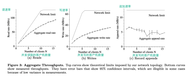
Figure 3: Aggregate throughput: The top curve shows the upper limit of the aggregate theoretical throughput for our network topology. The lower curve shows the observed throughput. This curve has 95% reliability because sometimes the measurements are not precise enough.

Figure 3(a) shows the overall read speed of N clients and the theoretical limit of this speed. When the 1Gbps link connecting the two switches is saturated, the overall read speed reaches a theoretical limit of 125MB/S, or 12.5MB/s per client when the 100Mbps NIC configured for each client is saturated. 80% of the theoretical read speed limit of the client. For 16 clients, the overall read speed reaches 94MB/s, which is about 75% of the theoretical overall read speed limit, i.e., 6MB/s per client. The overall read efficiency decreases.

6.1.2 Writing

N clients write data to N different files at the same time. Each client writes 1GB of data continuously at a rate of 1MB per write. Figure 3(b) shows the overall write speeds and their theoretical limits. The theoretical limit is 67MB/s because we need to write each byte to 3 of the 16 Chunk servers, and the input connection speed of each Chunk server is 12.5MB/s.

The write speed for one client is 6.3MB, which is roughly half of the theoretical limit. The main reason for this result is our network stack. It is not compatible with the pipeline model we use when pushing data to the Chunk server. The data transfer delay from one replica to another reduces the overall write speed.

The overall write speed for 16 clients reached 35MB/s (i.e. 2.2MB/s per client), which is only about half of the theoretical limit. Similar to the case of multiple clients reading, as the number of clients increases, the chance of multiple clients writing to the same Chunk server at the same time increases. Moreover, 16 clients writing in parallel can cause much more conflict than 16 clients reading in parallel, because each write involves three different copies.

Writes are slower than we thought. In practice, this did not become a major problem for us because even if the latency could be felt on a single client, it would not have a significant impact on the overall write bandwidth when there are a large number of clients.

6.1.3 Record Append

Figure 3(c) shows the performance of the record append operation. n clients append data to a file simultaneously. The performance of the record append operation is limited by the bandwidth of the Chunk server that holds the last Chunk of the file, independent of the number of clients. The speed of record appending starts at 6.0 MB/s for one client and decreases until 4.8 MB/s for 16 clients. The decrease in speed is mainly due to network congestion at different clients and the difference in network transmission speed.

Our program tends to process multiple such files at the same time. In other words, N clients append data to M shared files at the same time, where both N and M are tens or hundreds or more. So, in our real application, network congestion on the Chunk server does not become a serious problem, and if a file on the Chunk server is being written, the client will go and write another file.

6.2 Clusters in real-world applications

Let’s now take a closer look at two clusters that are being used within Google and are somewhat representative. Cluster A is typically used by hundreds of engineers for research and development. A typical task is to be manually initialized and then run for hours on end. It usually reads several MB to several TB of data, then transforms or analyzes it and finally writes the results back to the cluster. Cluster B is primarily used to process the current production data. The tasks in Cluster B last much longer, generating and processing terabytes of data sets continuously with little human intervention. In both cases, a single “task” refers to multiple processes running on multiple machines that read and write multiple files simultaneously.

6.2.1 Storage

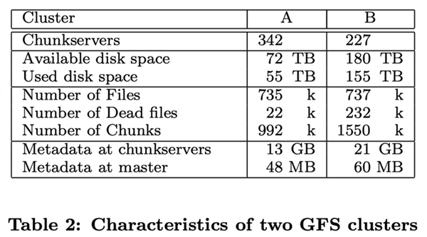
As described in the first five rows of the table above, both clusters consist of hundreds of Chunk servers supporting several terabytes of hard disk space; both clusters store a large amount of data but still have space left over. The “used space” contains all the Chunk copies. Virtually all files are copied in triplicate. Therefore, the clusters actually store 18TB and 52TB of file data each.

Both clusters store about the same number of files, but cluster B has a large number of dead files. A “dead file” is a file that has been deleted or replaced by a new version of the file, but the storage space has not yet been reclaimed. Since Cluster B stores a large number of files, it also has a large number of chunks.

6.2.2 Metadata

The Chunk server holds a total of more than a dozen GB of metadata, mostly Checksum from user data, in 64KB-sized chunks. other metadata held on the Chunk server is the version number information of the Chunk, which we described in section 4.5.

The metadata stored on the Master server is much smaller, about tens of MB, or an average of 100 bytes of metadata per file. This is the same as we envisioned, and the memory size of the Master server does not become a bottleneck in the capacity of the GFS system in practice. The metadata for most files is the filename stored in prefix-compressed mode. other metadata stored on the Master server includes the owner and permissions of the file, the file-to-Chunk mapping relationship, and the current version number of each Chunk. In addition, for each Chunk, we store the current copy location and a reference count to it, which is used to implement copy-on-write.

For each individual server, whether it is a Chunk server or a Master server, only 50MB to 100MB of metadata is stored. Therefore, recovering the server is very fast: it only takes a few seconds to read this data from disk before the server responds to a client request. However, the Master server will continue to bounce around for a while-usually 30 to 60 seconds-until it finishes polling all the Chunk servers and gets information about the location of all the Chunks.

6.2.3 Read and Write Rates

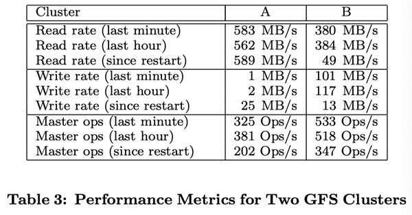
Table III shows the read and write rates for different time periods. At the time of testing, both clusters had been running for about a week. (Both clusters had recently been restarted due to upgrading to a new version of GFS.) After the clusters were restarted, the average write rate was less than 30MB/s. When we extracted the performance data, the clusters were running at the same time.

When we extracted the performance data, Cluster B was doing a lot of writes, with a write rate of 100MB/s, and a network load of 300MB/s due to three copies of each Chunk.

The read rate is much higher than the write rate. As we envisioned, the percentage of the total workload is much higher for reads than for writes. Both clusters are performing heavy read operations. In particular, Cluster A maintained a read rate of 580 MB/s for a week. Cluster A’s network configuration can support 750MB/s, which is clearly an efficient use of resources. Cluster B supports a peak read speed of 1300MB/s, but its application only uses 380MB/s.

6.2.4 Master server load

The data in Table 3 shows that the number of operation requests sent to the Master server is about 200 to 500 per second. the Master server can easily handle this request rate, so the processing power of the Master server is not the bottleneck of the system.

In earlier versions of GFS, the Master server was occasionally the bottleneck. It spent most of its time sequentially scanning a very large directory (containing tens of thousands of files) for a particular file. So we modified the data structure of the Master server to improve efficiency by performing a dichotomous lookup of the namespace. Now the Master server can easily perform thousands of file accesses per second. If needed, we can further increase the speed by setting up name lookup buffers before the namespace data structure.

6.2.5 Recovery Time

When a Chunk server fails, the number of some Chunk copies may be lower than the number specified by the replication factor, and we must bring the number of Chunk copies up to the number specified by the replication factor by cloning copies. The time taken to recover all Chunk copies depends on the number of resources. In our experiment, we Kill one of the Chunk servers on cluster B. This Chunk server has about 15,000 Chunks on it, totaling 600 GB of data. To minimize the impact of cloning operations on running applications and to provide correction space for GFS scheduling decisions, we set the number of concurrent cloning operations in the cluster to 91 by default (40% of the number of Chunk servers), with a maximum allowed bandwidth of 6.25MB/s (50mbps) per cloning operation. All Chunk was recovered in 23.2 minutes with a replication rate of up to 440MB/s.

In another test, we Kill off two Chunk servers, each with approximately 16,000 Chunks, for a total of 660GB of data. These two failures resulted in 266 Chunks with only a single copy. These 266 Chunks were replicated by GFS priority scheduling and recovered to have at least two copies within 2 minutes; the cluster is now brought to another state where the system can tolerate the failure of another Chunk server without losing data.

6.3 Workload Analysis (Workload Breakdown)

In this section, we show a detailed analysis of the workload situation of two GFS clusters, which are similar to, but not identical to, those in Section 6.2. Cluster X is used for research and development, and cluster Y is used for production data processing.

6.3.1 Methodology and Notes

These result data listed in this section include only the raw requests initiated by the client, and therefore reflect the full workload generated by our application on the GFS file system. They do not include requests that interact between servers to fulfill client requests, nor do they include requests related to background activities within GFS, such as forward-forwarded write operations, or operations such as reload balancing.

We derive reconstructed statistical information about IO operations from the real RPC request logs recorded by the GFS server. For example, a GFS client program may split a read operation into several RPC requests to increase parallelism, and we can derive the original read operation from these RPC requests. Because our access model is highly programmatic, we consider any data that does not match to be an error. Applications that log more exhaustively have the potential to provide more accurate diagnostic data; but it is impractical to recompile and restart thousands of running clients for this purpose, and it is a heavy workload to collect results from that many clients.

Over generalization from our workload data should be avoided. Because Google has full control over GFS and the applications that use it, the applications are optimized for GFS and, at the same time, GFS is designed for those applications. Such interactions may also exist in programs and file systems in general, but in our case the impact of such interactions may be more significant.

6.3.2 Chunk server workload

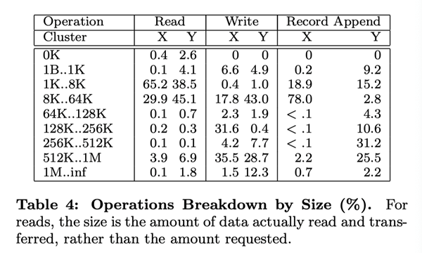
Table 4 shows the distribution of operations according to the size of the data volume involved. The read operations show a bimodal distribution by the size of the data volume involved in the operation. Small read operations (less than 64KB) are generally initiated by the client of the lookup operation, aiming to find small chunks of data from huge files. Large read operations (greater than 512KB) are generally performed by reading the entire file sequentially from start to finish.

On cluster Y, a significant number of read operations do not return any data. In our applications, especially in production systems, files are often used as producer-consumer queues. The producer appends data to the file in parallel, while the consumer reads data from the end of the file. In some cases, the consumer reads faster than the producer writes, which can lead to a situation where no data is read. Cluster X is typically used for short data analysis tasks rather than long-running distributed applications, so this is rarely the case with Cluster X.

Write operations also show the same bimodal distribution by data size. Large write operations (over 256KB) are usually caused by Writer’s use of a caching mechanism, where Writer caches smaller data and writes it in bulk afterwards through frequent checkpoint or synchronization operations, or simply by counting the amount of data for small writes (less than 64KB).

Observe again the record append operation. We can see that cluster Y has a much larger percentage of large record append operations than cluster X. This is because cluster Y is used for our production system and is more fully tuned for GFS.

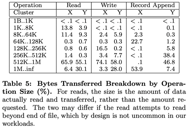
Table 5 shows the total data transfer volume by the size of the data volume involved in the operation. Among all the operations, the large operations (more than 256KB) take up the major amount of transfers. Smaller reads (less than 64KB), although transferring a relatively small amount of data, still account for a significant percentage of the reads, due to the workload of random Seek in the file.

6.3.3 Record Append vs. Write Operations

Record append operations are heavily used in our production system. For cluster X, the ratio of record append operations to normal write operations is 108:1 bytes to 8:1 operations, and for cluster Y, our production system, the ratios are 3.7:1 and 2.5:1, respectively. furthermore, this data set shows that record append operations are more prevalent than write operations on both of our clusters. For cluster X, the ratio of record append operations is lower throughout the measurement, so the results are influenced by one or two applications using certain buffer sizes.

As expected, our data modification operations are mainly record append operations rather than write operations in the overwrite mode. We measured data overwrite writes for the first copy. This approximates a client deliberately overwriting the data it has just written, rather than adding new data. For cluster X, the ratio of overwrite writes to bytes occupied by write operations is less than 0.0001%, and the ratio to the number of operations occupied is less than 0.0003%. For cluster Y, both of these ratios are 0.05%. Although this is only for a particular slice, it is still higher than we would expect. This is due to the fact that most of these overwritten writes are due to retry cases after errors or timeouts on the client side. This should not be counted as part of the workload in nature, but rather as a result of the retry mechanism.

6.3.4 Master’s workload

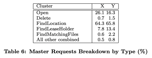
Table 6 shows the breakdown of the requests on the Master server by type. Most of the requests are read operations querying Chunk location information (FindLocation), and modify operations querying the information of the lease-holder (FindLease-Locker).

Cluster X and Y differ significantly in the number of deletion requests because cluster Y stores production data and generally regenerates data and replaces old data with new versions of data. The difference in number is also hidden in the Open request, since older versions of files may be implicitly deleted when opened in rewrite mode (similar to the “w” mode in UNIX’s open function).

FindMatchingFiles is a pattern matching request that supports “ls” and other similar file system operations. Unlike other requests from the Master server, it can retrieve most of the namespace, and is therefore a very expensive operation. Cluster Y has more of these requests because the automated data processing task process needs to examine various parts of the file system to get a global view of the state of the application. In contrast, applications in cluster X tend to be more controlled by individual users and usually know in advance the names of all the files they need to use.

7. Experience

During the process of building and deploying GFS, we experienced a variety of problems, some operational and some technical.

Initially, GFS was envisioned as a back-end file system for our production systems. Over time, support for research and development tasks was gradually added to the use of GFS. We started adding minor features such as permissions and quotas, and by now, GFS had initial support for these features. While our production system is tightly controlled, this is not always the case at the user level. More infrastructure is needed to prevent users from interfering with each other.

Our biggest problem is with disks and the problems associated with Linux. Many disks claim that they support a certain range of Linux IDE hard drive drivers, but this is not reflected in real world applications, which only support the latest drivers. Because the protocol versions are close, most disks will work, but occasionally there is a protocol mismatch that causes the driver and kernel to misjudge the state of the drive. This can lead to data being accidentally corrupted due to problems in the kernel. This problem led us to use Checksum to verify the data, and we also modified the kernel to handle these protocol mismatches.

Earlier, we encountered some problems with the Linux 2.2 kernel, mainly with the efficiency of fsync(). Its efficiency was related to the size of the file rather than the size of the modified part of the file. This gave us problems when our operation log files were too large, especially when we had not implemented Checkpoint yet. We went to great lengths to solve this problem with synchronous writing, but finally ported to the Linux 2.4 kernel.

Another Linux-related problem was the single read/write lock problem, meaning that any thread in a given address space had to hold first when page in from disk (read lock) or rewrite the address space when mmap() was called (write lock). We found that we had occasional timeouts even when our system was lightly loaded, and we spent a lot of effort looking for resource bottlenecks or hardware problems. We finally found that this single lock was locking the current network thread while the disk thread was swapping previously mapped data to disk, preventing it from mapping the new data to memory. Since our performance was mostly limited by the network interface and not the bandwidth of the memory copy, we solved this problem by replacing mmap() with pread(), using an additional copy action.

Despite occasional problems, Linux’s open source code allows us to quickly explore and understand the system’s behavior. In due course, we will improve the kernel and share these changes with the open source community.

8. Related work

Similar to other large distributed file systems, such as AFS [5], GFS provides a location-independent namespace, which allows data to be transparently migrated across locations for purposes such as load balancing or disaster redundancy. Unlike AFS, GFS distributes files to different servers in a manner more similar to Xfs [1] and Swift [3], which is designed to improve overall performance and disaster redundancy.

Since disks are relatively cheap and replication is much simpler than the RAID [9] approach, GFS currently uses only replication for redundancy and thus takes up more bare storage space than xFS or Swift .

Unlike file systems such as AFS, xFS, Frangipani [12], and Intermezzo [6], GFS does not provide any Cache mechanism at the file system level. Our main work hardly reads data repeatedly when a single application executes, because they work either by streaming a large dataset or by randomly Seeking to a location in a large dataset and later reading a small amount of data at a time.

Some distributed file systems, such as Frangipani, xFS, Minnesota’s GFS [11], and GPFS [10], remove the central server and rely only on distributed algorithms to ensure consistency and manageability. We chose the central server approach in order to simplify the design, increase reliability, and be able to scale flexibly. In particular, it is worth mentioning that since the centrally located Master server keeps almost all the Chunk-related information and controls all the changes of Chunk, it greatly simplifies the implementation of the otherwise very complex Chunk allocation and replication policy. We ensure disaster redundancy by reducing the amount of state information kept by the Master server and by replicating the state of the Master server to other nodes. Scalability and high availability (for reads) are currently guaranteed through our shadow Master server mechanism. Changes to the Master server state are persisted by means of pre-written logs. For this purpose, we can adapt to use a primary-copy scheme similar to that in Harp [7], thus providing tighter consistency guarantees than our current scheme.

We solve a puzzle that is similar to the one encountered by Lustre [8] in how to guarantee the overall performance of the system when there are a large number of clients. However, we achieve the goal of simplifying the problem by focusing only on the needs of our application, rather than providing a POSIX-compatible file system. In addition, the GFS design anticipates clustering with a large number of unreliable nodes, so a disaster redundancy scheme is at the core of our design.

GFS is very similar to the NASD architecture, which is based on network disks, while GFS uses ordinary computers as Chunk servers, just like the original NASD solution. The difference is that our Chunk server uses an inert allocation of fixed-size Chunks instead of allocating variable-length object storage space. In addition, GFS implements features such as reload balancing, replication, and recovery mechanisms that are needed in a production environment.

Unlike Minnesota’s GFS and NASD, we do not change the storage device model, and we focus on using common devices to solve the daily data processing of very complex distributed systems.

We implement a producer-consumer queue through atomic record appending operations, a problem similar to the distributed queue in River [2].River uses a cross-host, memory-based distributed queue, for which the data flow must be carefully controlled, while GFS is implemented as a persistent file that can be concurrently appended by producers.The River model Supports distributed queues from m- to -n, but lacks the fault tolerance provided by persistent storage; GFS only supports queues from m- to -1. Multiple consumers can read a file at the same time, but the intervals of their input streams must be aligned.

9. concluding remarks

The Google File System demonstrates the qualities of a system that uses common hardware to support large-scale data processing. While some of the design points are tailored to our particular needs, there are many features that are applicable to data processing tasks of similar size and cost.

First, we evaluated the characteristics of a traditional file system against our current and anticipated future application size and technology environment. The results of our evaluation lead us to a design philosophy that uses a completely different approach than the traditional one. According to our design philosophy, we consider component failures to be the norm rather than anomalies, optimize for large files that are written using appending (potentially concurrent appending) and then read (usually serialized reads), and improve the overall system by extending the standard file system interface and relaxing interface restrictions.

Our system provides disaster redundancy through continuous monitoring, replication of critical data, and rapid and automatic recovery. Chunk replication allows us to be fault-tolerant to Chunk server failures. The high frequency of component failures requires the system to have an online repair mechanism that can periodically and transparently repair corrupted data, as well as recreate lost copies at the first opportunity. In addition, we use Checksum to detect data corruption at the disk or IDE subsystem level, which is quite high in such a large system with a staggering number of disks.

Our design ensures that we can provide high aggregate throughput when there are a large number of concurrent read and write operations. We achieve this by separating the control flow from the data flow, with the control flow handled at the Master server and the data flow handled at the Chunk server and clients. When general operations involve the Master server, these measures minimize the burden on the Master server due to the larger Chunk size chosen by GFS and the handover of control to the master replica via Chunk Lease. This keeps a simple, central Master from becoming a bottleneck. We believe our optimization of the network stack can improve the current write throughput limits for per-client.

GFS has successfully fulfilled our storage needs and is widely used within Google, both as a storage platform for research and development, and as a data processing platform for production systems. It is an important tool for our continued innovation and for dealing with difficult problems across the WEB.

GFS System Explained

Benefits of GFS

• master and chunkserver design, separating file management and file storage
• Split file storage into chunks for concurrent access and higher throughput
• Separate control flow and data flow when modifying data, making full use of each machine’s bandwidth
• Use lease to reduce master workload and prevent split-brain problem
• Optimized for file appending and sequential reads
• Good fault tolerance

Disadvantages of GFS

• Only one master, if there is too much metadata, memory may not be enough
• One master can be overloaded if the client volume is large
• master can’t restart automatically in case of error, so it is time consuming to switch master manually after failure
• master is too inefficient in garbage collection by browsing all chunks
• Not good at handling random write problem, large amount of small file storage
• Consistency is too loose to handle tasks that require high consistency
• GFS is designed for systems running in a single data center