Big Data Fundamentals: Hadoop

This first article was organized in 2014, in this 7~8 years time, Hadoop has changed a lot, but the most core content has not changed so much, the article at that time still has some reference significance. Once again, we will re-do the organization.

An overview of Hadoop

Hadoop, a distributed system infrastructure, was developed by the Apache Foundation. Users can develop distributed programs without understanding the underlying details of distribution. Leverage the power of clusters for high-speed computing and storage. Simply put, Hadoop is a software platform that can be more easily developed and run to handle large-scale data. The platform is implemented using Java, an object-oriented programming language, and has good portability.

History of Hadoop

On September 4, 1998, Google Inc. was founded in Silicon Valley as an Internet search engine that needed to store a large number of web pages and continuously optimize its search algorithms to improve search efficiency. in 2003, Google published a technical academic paper that publicly introduced its Google File System (GFS). This is a special file system designed by Google to store huge amount of search data. The following year, in 2004, Doug Cutting implemented a distributed file storage system based on Google’s GFS paper, and named it NDFS (Nutch Distributed File System)

Still in 2004, Google published another technical academic paper introducing its own MapReduce programming model. This programming model, used for parallel analysis operations on large-scale data sets (>1TB). The following year (2005), Doug Cutting implemented it again in the Nutch search engine, based on MapReduce.

In 2006, the then still very powerful Yahoo (Yahoo) company, recruited Doug Cutting.

Here to add to explain the background of Yahoo recruiting Doug: before 2004, as the Internet pioneer Yahoo, is using Google search engine as its own search service. In 2004, Yahoo gave up Google, began to develop their own search engine. So….

After joining Yahoo, Doug Cutting upgraded NDFS and MapReduce and renamed it Hadoop (NDFS was also renamed HDFS, Hadoop Distributed File System).

This, later on, is the origin of the big-name big data framework system - Hadoop. The name Hadoop is actually the name of Doug Cutting’s son’s yellow toy elephant. So, the logo of Hadoop is a running yellow elephant.

Still in 2006, Google published another paper. This time, they introduced their own BigTable. This is a distributed data storage system, a non-relational database for handling massive amounts of data.

Doug Cutting, of course, did not let go and introduced BigTable inside his own hadoop system, and named it HBase.

So, the core part of Hadoop basically has the shadow of Google.

In January 2008, Hadoop successfully made its way to the top and officially became the top project of Apache Foundation. In February of the same year, Yahoo announced that it had built a Hadoop cluster with 10,000 cores and deployed its own search engine product on it. in July, Hadoop broke the world record as the fastest system for sorting 1TB of data, taking 209 seconds. Since then, Hadoop has entered a period of rapid development until now.

Hadoop 1.0

Hadoop is a software platform for developing and running large-scale data processing, and is an Apache open source software framework implemented in JAVA language to achieve distributed computing of massive amounts of data in a cluster of a large number of computers. MapReduce provides the computation of data, HDFS provides the storage of large amounts of data.

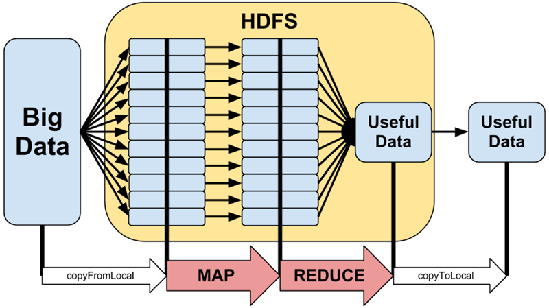
The idea of MapReduce is mentioned in a Google paper and has been widely circulated, and in a simple sentence MapReduce is “the decomposition of tasks and the aggregation of results”. HDFS stands for Hadoop Distributed File System, which provides the underlying support for distributed computing storage.

MapReduce

MapReduce can be roughly seen from its name, two verbs Map and Reduce, “Map” is to decompose a task into multiple tasks, “Reduce” is the decomposition of The results of the multi-tasking process are aggregated to produce the final analysis. Whether in the real world or in programming, a task can often be split into multiple tasks, and the relationship between tasks can be divided into two types: one is unrelated tasks, which can be executed in parallel; the other is the interdependence between tasks, and the order cannot be reversed, which cannot be processed in parallel.

In a distributed system, a cluster of machines can be regarded as a pool of hardware resources, and the parallel tasks can be split and then handed over to each free machine resource for processing, which can greatly improve the computational efficiency, while this resource-independence, for the expansion of the computing cluster undoubtedly provides the best design guarantee. After the task is broken down and processed, the results are then aggregated, which is what Reduce does.

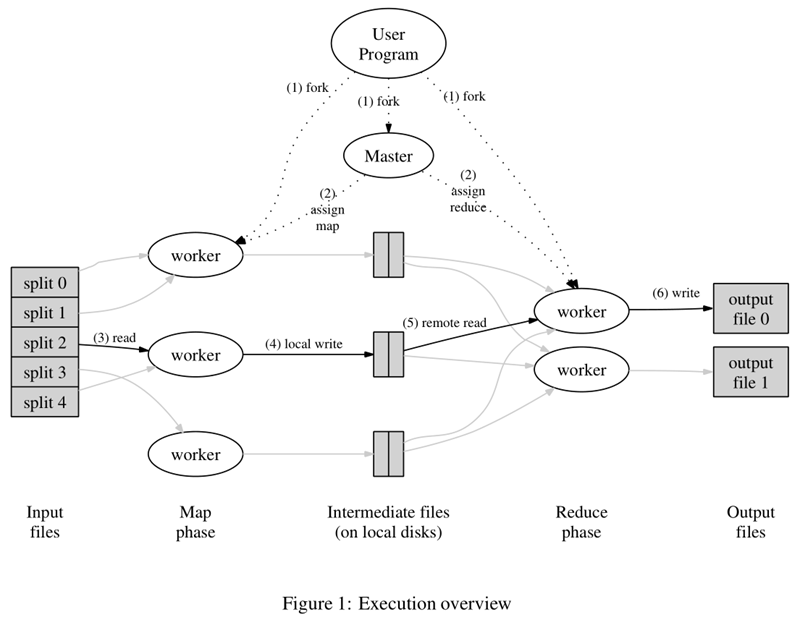
The diagram above is the flowchart given in the paper. Everything starts with the User Program at the top, which links to the MapReduce library and implements the most basic Map functions and Reduce functions. The order of execution is marked with numbers in the diagram.

• The MapReduce library first divides the user program’s input file into M copies (M is user-defined), each of which is typically 16MB to 64MB, as shown on the left side of the figure, into splits 0 to 4; then it uses fork to copy the user process to other machines in the cluster.
• The master is responsible for scheduling and assigning jobs (Map jobs or Reduce jobs) to idle workers, and the number of workers can be specified by the user.
• The number of Map jobs is determined by M and corresponds to split. The Map job extracts the key-value pairs from the input data, and each key-value pair is passed to the map function as an argument.
• The cached intermediate key-value pairs are periodically written to local disk and are divided into R zones, the size of which is user-defined, and each zone will correspond to a Reduce job in the future; the location of these intermediate key-value pairs is communicated to master, which is responsible for forwarding the information to the Reduce worker.
• The master informs the worker who assigned the Reduce job where the partition it is responsible for is located (there must be more than one place; each Map job generates intermediate key-value pairs that may map to all R different partitions), and when the Reduce worker reads all the intermediate key-value pairs it is responsible for, it first sorts them so that key-value pairs with the same key are clustered together. Since different keys may map to the same partition, i.e., the same Reduce job (who wants fewer partitions?), sorting is necessary.
• The reduce worker iterates over the sorted intermediate key-value pairs, and for each unique key, passes the key and associated value to the reduce function, which produces output that is added to the output file for that partition.
• When all Map and Reduce jobs are done, the master wakes up the genuine user program and the MapReduce function calls the code that returns the user program.

After all executions are complete, the MapReduce output is placed in R partitioned output files (each corresponding to a Reduce job). The user does not usually need to merge these R files, but instead gives them as input to another MapReduce program. In the whole process, the input data is from the underlying distributed file system (HDFS), the intermediate data is placed on the local file system, and the final output data is written to the underlying distributed file system (HDFS). And we should note the difference between a Map/Reduce job and a map/reduce function: a Map job processes a partition of input data and may need to call the map function several times to process each input key-value pair; a Reduce job processes an intermediate key-value pair of a partition, during which the reduce function is called once for each different key, and the Reduce job eventually corresponds to an output file as well.

The appeal process is divided into three phases. The first phase is the preparation phase, including 1 and 2, where the MapReduce library is the main character, completing tasks such as splitting the job and copying the user program; the second phase is the run phase, including 3, 4, 5, and 6, where the main characters are the user-defined map and reduce functions, and each small job is running independently; the third phase is the sweep phase, when the job is completed and the results are placed in the output file It is up to the user what to do with the output.

Before the Map, there may be a Split process for the input data to ensure task parallelism, and after the Map, there will be a Shuffle process to improve the efficiency of Reduce and reduce the pressure of data transfer. The Shuffle process is the core of MapReduce, and is also known as the place where the magic happens. To understand MapReduce, Shuffle is a must.

MapReduce’s Shuffle Process

The Shuffle process in MapReduce is more like the reverse of shuffle, converting a set of irregular data into a set of data with certain rules as much as possible. Why does the MapReduce computing model need the Shuffle process? We all know that the MapReduce computing model generally consists of two important phases: Map is the mapping, which is responsible for filtering and distributing the data; Reduce is the statute, which is responsible for computing and merging the data. data in Reduce comes from Map, and the output of Map is the input of Reduce, which needs Shuffle to get the data.

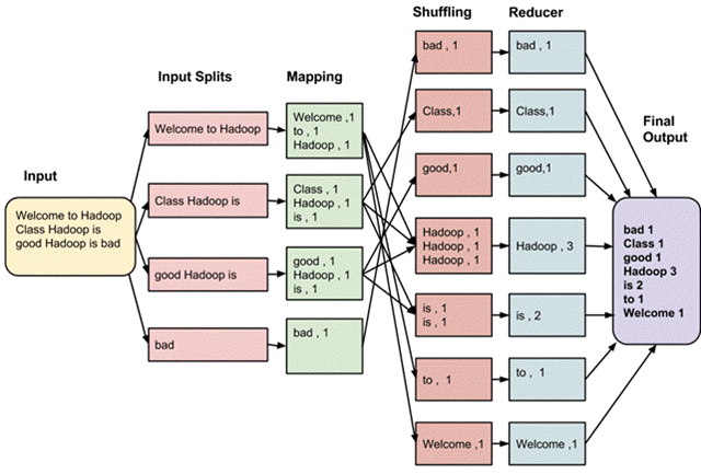
Probably you are more familiar with the Collections.shuffle(List) method in the Java API, which randomly disrupts the order of the elements in the argument list. If you don’t know what Shuffle is in MapReduce, then look at this diagram.

In fact, the intermediate process is called MapReduce Shuffle, which starts from the last call in the map() method of the Map Task task, i.e., the output of intermediate data, and ends when the Reduce Task task starts to execute the reduce() method. The shuffle process is divided into two phases: the Map side shuffle phase and the Reduce side shuffle phase.

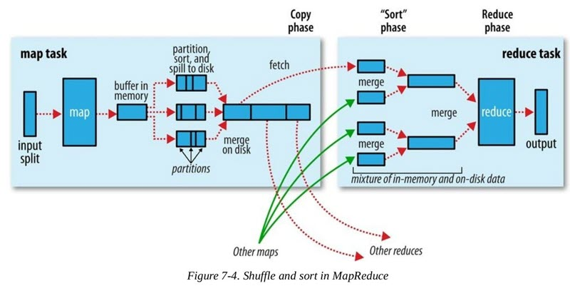
The whole process from Map output to Reduce input can be broadly called Shuffle. shuffle spans both Map side and Reduce side, including the Spill process on the Map side and the copy and sort processes on the Reduce side, as shown in the figure.

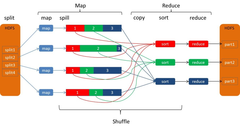
The Spill process includes the steps of output, sorting, overwriting, and merging, as shown in the figure.

1. Collect phase

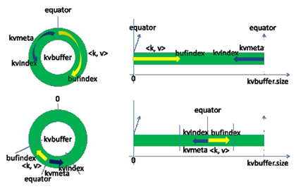
Each Map task continuously outputs data in the form of <key, value> pairs into a ring data structure constructed in memory. The ring data structure is used to make more efficient use of memory space by placing as much data in memory as possible. This data structure is actually a byte array called Kvbuffer, as the name implies, but it contains not only <key, value> data, but also some index data, giving the area where the index data is placed the alias Kvmeta, and putting an IntBuffer (the byte order is the platform’s own byte order) on top of an area of Kvbuffer. ). The <key, value> data region and the index data region are two adjacent and non-overlapping regions in the Kvbuffer, and are divided by a demarcation point that is not constant, but is updated after each Spill. The initial demarcation point is 0. The <key, value> data is stored in the upward direction, and the index data is stored in the downward direction, as shown in the figure.

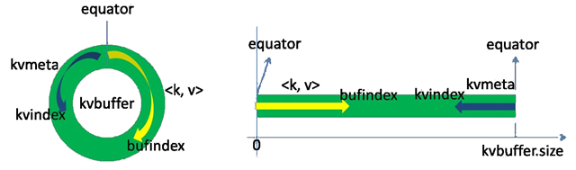
Kvbuffer’s storage pointer bufindex is always bored upward, for example, bufindex initial value is 0, after an Int-type key is written, bufindex grows to 4, after an Int-type value is written, bufindex grows to 8.

The index is the index of <key, value> in the kvbuffer, a quadruple, including: the starting position of value, the starting position of key, partition value, length of value, occupying four Int lengths, Kvmeta’s storage pointer Kvindex is jumping down four “grids” each time “, and then fill the data of the quadruplet one grid at a time upwards. For example, the initial position of Kvindex is -4. After the first <key, value> is written, the position of (Kvindex+0) holds the starting position of value, the position of (Kvindex+1) holds the starting position of key, the position of (Kvindex+2) holds the value of partition, the position of (Kvindex+3) holds the length of value, and then the position of Kvindex+2 holds the length of partition. then Kvindex jumps to -8, and after the second <key, value> and index are written, Kvindex jumps to -32.

Although the size of Kvbuffer can be set by parameters, it is only that big in total, and the <key, value> and index keep increasing. The process of brushing data from memory to disk and then writing data to memory is called Spill, how clear is the name?

About the conditions for Spill trigger, that is, the extent to which the Kvbuffer used to start Spill, or to speak a little. If the Kvbuffer is used up to the point where no space is left before starting Spill, then the Map task will need to wait for Spill to finish freeing up space before it can continue writing data; if the Kvbuffer is only full to a certain extent, such as 80% when it starts Spill, then the Map task can continue writing data while Spill is in progress, and if If Spill is fast enough, Map may not even need to worry about free space. The latter is generally chosen as the greater of the two benefits.

Spill this important process is undertaken by the Spill thread, Spill thread from the Map Task received the “command” after the official work, dry work called SortAndSpill, it turns out that not only Spill, before Spill there is a controversial Sort.

In the Map Task task business processing method map(), the last step through OutputCollector.collect(key,value) or context.write(key,value) output Map Task intermediate processing results, in the related collect(key, value) method, the Partitioner.getPartition(K2 key, V2 value, int numPartitions) method will be called to obtain the partition number corresponding to the output key/value (the partition number can be considered as corresponding to a node to execute the Reduce Task), and then the <key,value,partition> is temporarily stored in memory in a circular data buffer inside MapOutputBuffe, which has a default size of 100MB and can be resized with the parameter io.sort.mb.

When the data usage in the buffer reaches a certain threshold, a Spill operation is triggered to write part of the data in the ring buffer to disk, generating a temporary spill file of Linux local data; then after the buffer usage reaches the threshold again, a spill file is generated again. Until the data is processed, many temporary files will be generated on disk.

The data stored inside MapOutputBuffer uses a two index structure involving three ring memory buffers. The following is a look at the two-level index structure.

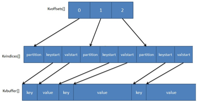
Three ring buffers.

• The kvoffsets buffer, also called the offset index array, is used to store the offset of key/value information in the location index kvindices. When the usage of kvoffsets exceeds sort.spill.percent (default is 80%), it triggers an “overwrite” operation of the SpillThread thread, i.e., it starts a Spill phase operation.
• kvindices buffer, also called position index array, is used to store the starting position of the key/value in the data buffer kvbuffer.
• kvbuffer, the data buffer, is used to hold the actual key/value values. By default this buffer can use up to 95% of sort.mb. When the kvbuffer usage exceeds io.sort.spill.percent (80% by default), a SpillThread “overwrite” operation will be started, which means that a Spill phase operation.

2、Sort stage

First sort the data in Kvbuffer in ascending order according to the partition value and key two keywords, moving only the index data, sorting results in Kvmeta data gathered together according to partition as a unit, the same partition in accordance with the key order.

3. Spill phase

When the buffer usage reaches a certain threshold, an “overwrite” operation is triggered to write part of the data in the ring buffer to the Linux local disk. It is important to note that before writing data to disk, the data to be written to disk will be sorted by partition partition number in <key,value,partition>, then by key, and if necessary, for example, if Combiner is configured and the current system load is not very high, the data with the same partition partition number and key will be sorted. If necessary, for example, if Combiner is configured and the current system load is not very high, data with the same partition partition number and key will be aggregated, and if the configuration is set and the intermediate data is compressed, compression will be done as well.

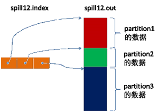
The spill thread creates a disk file for the spill process: it looks for a directory that can store this much space from all local directories in turn and creates a file like “spill12.out” in it after finding it. Spill thread spits <key, value> data into this file one by one according to the ordered Kvmeta partition, and spits the next partition in order after the data of one partition is spit out, until all the partitions are traversed. The data corresponding to a partition in the file is also called segment.

All the data corresponding to the partitions are placed in this file, although they are stored in order, but how to directly know the starting position of a partition stored in this file? The powerful index comes into play again. There is a triplet to record the index of the data corresponding to a partition in this file: the starting position, the original data length, and the compressed data length, one partition corresponds to one triplet. Then these index information is stored in memory, if the memory can not be put, the subsequent index information needs to write to the disk file: from all the local directory training to find the directory that can store such a large space, and after finding it, create a file similar to “spill12.out.index” in it This file stores not only the index data, but also the crc32 checksum data. (spill12.out.index is not necessarily created on disk, if memory (default 1M space) can be put in memory, even if it is created on disk, and spill12.out file may not be in the same directory.)

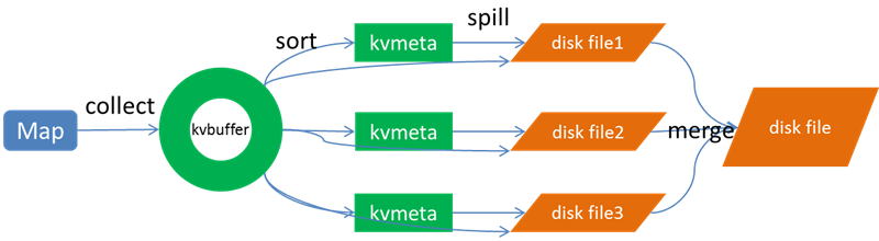
Each Spill process generates at least one out file, and sometimes an index file, and the number of Spills is also branded in the file name. The correspondence between the index file and the data file is shown in the following figure.

Map still writes data to kvbuffer, so the question arises: <key, value> is just bored with growing upwards according to bufindex pointer, while kvmeta is just growing downwards according to Kvindex. The kvmeta is only growing downwards according to the Kvindex, should we keep the starting position of the pointer unchanged and keep running, or find another way? If we keep the starting position of the pointer unchanged, soon bufindex and Kvindex will meet, and it is undesirable to restart or move the memory after the meeting. map takes the middle position of the remaining space in kvbuffer and sets this position as the new demarcation point, bufindex pointer moves to this demarcation point and Kvindex moves to -16 of this demarcation point. Then the two can harmoniously place data according to their established trajectory, and when Spill is finished and space is freed up, no changes need to be made to move on. The conversion of the demarcation points is shown in the following figure.

The Map task always writes the output data to disk, and even if the amount of output data is small enough to fit all in memory, it will still swipe the data to disk at the end.

4、Combine phase

After all the data of the Map Task tasks have been processed, a merge operation will be done on all the intermediate data files generated by the tasks to ensure that a Map Task will eventually generate only one intermediate data file.

**5. Copy stage. **

The Reduce task drags the data it needs to the individual Map tasks via HTTP. Each node starts a resident HTTP server, and one of its services is to respond to the Reduce dragging Map data. When a MapOutput HTTP request comes in, the HTTP server reads the data in the corresponding Map output file corresponding to this Reduce part and outputs it to Reduce via a network stream.

The Reduce task drags the data corresponding to a Map, and writes the data directly to memory if it can fit in memory, and Reduce drags the data to each Map, and each Map corresponds to a piece of data in memory. merge output to a file on disk.

If the Map data cannot fit in the memory, the Map data is written directly to the disk by creating a file in the local directory, reading the data from the HTTP stream and writing it to the disk, using a buffer size of 64 K. Dragging a Map data over creates a file, and when the number of files reaches a certain threshold, it starts a disk file merge to merge these files into one file. When the number of files reaches a certain threshold, a disk file merge is started, merging these files into a single file.

Some Map data is small enough to be placed in memory, and some Map data is large enough to be placed on disk, so that in the end, some of the data dragged by the Reduce task is placed in memory and some is placed on disk, and finally a global merge is performed on these.

By default, JobTracker will start scheduling the execution of the Reduce Task task when the number of all executed Map Task tasks for the whole MapReduce job exceeds 5% of the total number of Map Task. Then the Reduce Task task starts mapred.reduce.parallel.copies by default (default is 5), and each of the MapOutputCopier threads copies a copy of its own data to the completed Map Task task nodes. The copied data is first saved in the memory buffer, and then written to disk when the in-flush buffer usage reaches a certain threshold.

6. Merge Phase

While copying data remotely, the Reduce Task starts two background threads in the background to do merge operations on the data files in memory and on disk to prevent too much memory usage or too many files born on disk.

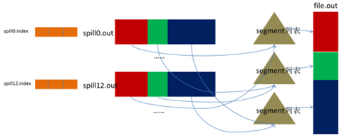
The Map Task may perform several spills if the output data volume is large, and out files and Index files will be generated a lot and distributed on different disks. Finally the merge process, which merges these files, shines through.

How does the merge process know where all the generated Spill files are located? How does the merge process know the index information of the spill files? Yes, it also scans all the local directories to get the Index file and stores the index information in a list. Here, we encounter another puzzling point. In the previous Spill process, why not store the information in memory directly, why this extra step of scanning operation? In particular, the index data of Spill, which was previously written to disk when the memory limit was exceeded, now has to be read out from disk again, or needs to be loaded into more memory. The reason for this extra effort is that at this point kvbuffer, a memory hog, is no longer in use and can be recycled, and there is memory space to hold this data. (For richer people with more memory space, it is still worth considering using memory to skip these two io steps.)

Then create a file called file.out and a file called file.out.Index for the merge process to store the final output and index.

The output is merged partition by partition. For a partition, all index information corresponding to this partition is looked up from the index list and each corresponding segment is inserted into the segment list. That is, this partition corresponds to a segment list, and records the file name, starting position, length, etc. of the segment data corresponding to this partition in all the Spill files.

When this partition corresponds to many segments, the merging is done in batches: first, the first batch is taken out from the segment list and placed into the smallest heap with key as the key, and then each time the This merges the segments into a temporary segment and adds it back to the segment list; then the second batch is taken out from the segment list and merged into a temporary segment and added to the list; this is repeated until the remaining segments are a batch and output to the final file. .

The final index data is still output to the Index file.

This is the end of the Shuffle process at the Map side.

6、Merge Sort stage

When merging, sorting is also done. Since each Map Task has already done local sorting of the data, the Reduce Task only needs to do a merge sort to ensure the overall orderliness of the copy data. After performing the merge and sort operations, the Reduce Task passes the data to the reduce() method.

The Merge process is the same as the Merge process on the Map side, where the Map output is already ordered, and the Merge process is a merge sort, the so-called sort process on the Reduce side. Generally, Reduce is copy and sort at the same time, i.e., the two phases of copy and sort are overlapping rather than completely separate.

This is the end of the Shuffle process on the Reduce side.

HDFS

HDFS is the storage cornerstone of distributed computing, and Hadoop’s distributed file system has many similar qualities to other distributed file systems. A few basic characteristics of distributed file systems.

• A single namespace for the entire cluster.
• Data consistency. Suitable for a write-once-read-many model, where the client cannot see that a file exists until it has been successfully created.
• Files are split into multiple file blocks, each of which is assigned to a data node for storage and, depending on the configuration, is secured by replicated file blocks.

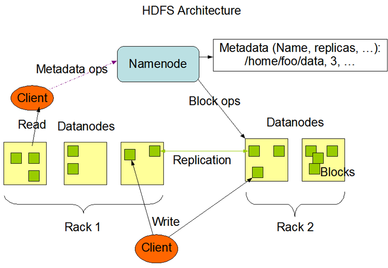
The above diagram shows three important roles of HDFS: NameNode, DataNode and Client. NameNode can be regarded as the manager of the distributed file system, mainly responsible for managing the file system namespace, cluster configuration information and replication of storage blocks. The DataNode is the basic unit of file storage, which stores the Block in the local file system, keeps the Meta-data of the Block, and periodically sends the information of all existing Blocks to the NameNode. The Client is the application that needs to get the distributed file system files. The interaction between them is illustrated here by three operations.

File write.

• Client initiates a file write request to the NameNode.
• The NameNode returns information to the Client about the DataNode it manages, based on the file size and the configuration of the file blocks.
• Client divides the file into multiple blocks and writes to each DataNode block in order according to the address information of the DataNode.

File Read.

• The Client initiates a file read request to the NameNode.
• NameNode returns information about the DataNode where the file is stored.
• Client reads the file information.

File Block Replication.

• The NameNode finds that some of the blocks of the file do not meet the minimum replication number or some of the DataNodes fail.
• Notify DataNode to replicate Blocks to each other.
• DataNode starts direct mutual replication.

Finally, a few more design features of HDFS (for framework design worth learning).

• Block placement: not configured by default. A Block will have three backups, one on the DataNode specified by the NameNode, another on the DataNode not on the same Rack as the specified DataNode, and the last on the DataNode on the same Rack as the specified DataNode. Backup is nothing but for data security, consider the failure of the same Rack and the performance of data copy between different Racks on this configuration.
• Heartbeat detects the health of the DataNode, and if problems are found, data backup is taken to ensure the security of the data.
• Data replication (scenario for DataNode failure, the need to balance the storage utilization of DataNode and the need to balance the pressure of DataNode data interaction, etc.): Here first, using the HDFS balancer command, you can configure a Threshold to balance the disk utilization of each DataNode. For example, if the Threshold is set to 10%, then when the balancer command is executed, the average value of disk utilization of all DataNodes will be counted first, and then if the disk utilization of a DataNode exceeds the average value of Threshold, then the blocks of this DataNode will be transferred to disk. This is very useful for new nodes to join.
• Data handoff: CRC32 is used for data handoff. In addition to the data written to the file block, it also writes the cross-check information, which needs to be cross-checked before reading in.
• NameNode is a single point: If it fails, the task processing information will be recorded in the local file system and the remote file system.
• Data pipelined writing: When a client wants to write a file to a DataNode, first the client reads a Block and then writes to the first DataNode, then the first DataNode is passed to the backup DataNode, until all the NataNodes that need to write this Block are successfully written, then the client will continue to start writing the next Block.
• Safe Mode: At the beginning of the distributed file system startup, there will be safe mode. When the distributed file system is in safe mode, the content in the file system is not allowed to be modified nor deleted until the end of safe mode. The safe mode is mainly for checking the validity of data blocks on each DataNode when the system starts, and also for copying or deleting some data blocks according to the policy necessary. Safe mode can also be entered by command during runtime. In practice, when the system starts to modify and delete files, there will also be an error message that safe mode does not allow modification, just wait for a while.

Hadoop 2.0

Hadoop 2.0 is a distributed system infrastructure from Apache that provides storage and computation for massive data. YARN is used for resource management.

Comparison of the architecture of Hadoop 1.0 and Hadoop 2.0.

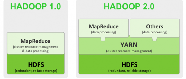
The main improvements in Hadoop 2.0 are.

• Implemented resource scheduling and management through YARN, so that Hadoop 2.0 can run more kinds of computing frameworks, such as Spark, etc.
• Implemented HA scheme for NameNode, that is, there are two NameNodes (one Active and the other Standby) at the same time, if the ActiveNameNode hangs, the other NameNode will switch to Active state to provide services, which ensures high availability of the whole cluster.
• HDFS federation is implemented. Since the metadata is placed in the memory of the NameNode, the memory limits the size of the whole cluster, and through HDFS federation, multiple NameNodes form a federation to jointly manage the DataNode, so that the cluster size can be expanded.
• Hadoop RPC serialization scales well by making the datatype module independent from RPC as an independent pluggable module.

YARN Basic Architecture

YARN is a resource manager for Hadoop 2.0. It is a general-purpose resource management system that provides unified resource management and scheduling for upper-layer applications. Its introduction brings great benefits to clusters in terms of utilization, unified resource management and data sharing.

The basic design idea of YARN is to split the JobTracker in Hadoop 1.0 into two independent services: a global resource manager ResourceManager and an application-specific ApplicationMaster for each application, where ResourceManager is responsible for resource management and allocation of the entire system, and ApplicationMaster is responsible for individual application resource management and allocation. The basic architecture is shown in the following figure.

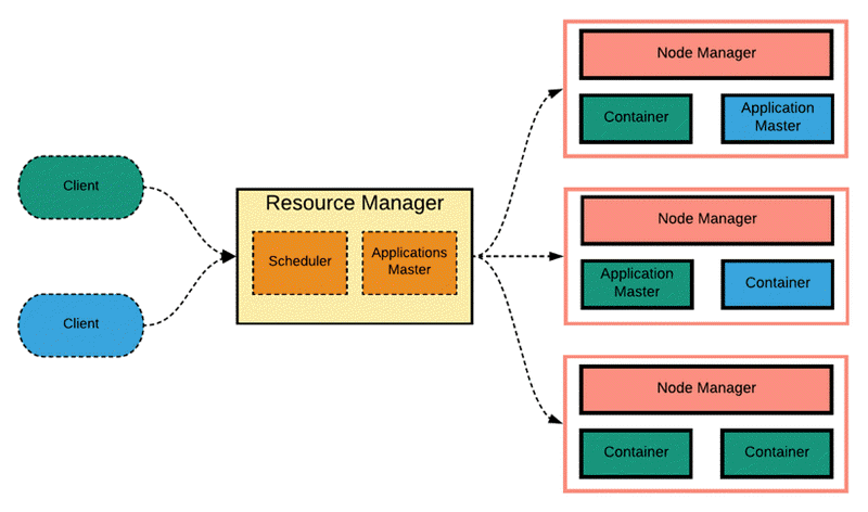
YARN is still a Master/Slave structure in general. ResourceManager is responsible for the unified management and scheduling of resources on each NodeManager. When a user submits an application, it is necessary to provide an ApplicationMaster for tracking and managing the application, which is responsible for requesting resources from the ResourceManager and asking the NodeManger to start tasks that can occupy certain resources. Since different ApplicationMaster are distributed to different nodes, they do not affect each other.

• ResourceManager: It is a global resource manager, responsible for resource management and allocation of the whole system, and mainly consists of two components: scheduler and application manager.
• Scheduler: It allocates the resources in the system to each running application based on capacity, queue, and other constraints. The scheduler allocates resources based on the resource requirements of the application only, and the resource allocation unit is represented by an abstract concept “Resource Container” (Container for short), which is a dynamic resource allocation unit that encapsulates resources such as memory, CPU, disk, network, etc., thus limiting the amount of resources used by each task. It is a dynamic resource allocation unit that encapsulates resources such as memory, CPU, disk, network, etc. to limit the amount of resources used by each task.
• Application Manager: Responsible for managing all applications throughout the system, including application submissions, negotiating resources with the scheduler to start the ApplicationMaster, monitoring the running status of the ApplicationMaster and restarting it in case of failure, etc.
• ApplicationMaster: Each application submitted by the user contains one ApplicationMaster. Its main functions include negotiating with the ResourceManager scheduler to obtain resources, further assigning the obtained tasks to internal tasks, communicating with the NodeManager to start/stop tasks, monitoring the running status of all tasks and restarting tasks by reapplying resources for them when they fail to run, etc.
• NodeManager: It is the resource and task manager on each node. It not only reports the resource usage and the running status of each Container on this node to ResourceManager regularly, but also receives and processes various requests from ApplicationMaster for Container start/stop, etc.
• Container: It is a resource abstraction in YARN, which encapsulates the multidimensional resources on a node, such as memory, CPU, disk, network, etc. When ApplicationMaster requests resources from ResourceManager, the returned resources are represented by Container. Container for each task, and the task can only use the resources described in that Container.

YARN workflow

When a user submits an application to Yarn, the main workflow of Yarn is as follows.

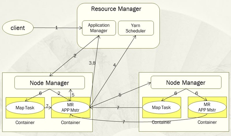
• Step 1, the user submits the application to Yarn, which includes the user program, related files, the start ApplicationMaster command, the ApplicationMaster program, etc.
• Step 2, the ResourceManager assigns the first Container to the application and communicates with the NodeManager where the Container is located and asks the NodeManager to start the ApplicationMaster corresponding to the application in this Container.
• Step 3, the ApplicationMaster first registers with the ResourceManager so that the user can view the running status of the application directly through the ResourceManager, and then it requests resources for each task ready for the application and monitors their running status until the end of the run, i.e., repeating the next steps 4~7.
• Step 4, ApplicationMaster uses polling to request and collect resources from ResourceManager via RPC protocol.
• Step 5, once the ApplicationMaster requests a resource, it communicates with the NodeManager corresponding to the requested Container and asks it to start a task in that Container.
• The NodeManager configures the runtime environment for the task to be started, including environment variables, JAR packages, binaries, etc., and writes the start command in a script through which the task is run.
• Step 7, each task reports its running status and progress to its corresponding ApplicationMaster via RPC protocol, so that the ApplicationMaster can keep track of the running status of each task, so that it can restart the task when it fails to run again.
• Step 8, after the application finishes running, its corresponding ApplicationMaster will communicate to the ResourceManager to request logging out and shutting itself down.

It is important to note that throughout the workflow, the ResourceManager and NodeManager are kept in touch through heartbeats, and the NodeManager reports the resource usage of its node to the ResourceManager through heartbeat information.