Big Data Basics: HIVE

Hive Introduction

Hive, implemented by Facebook and open source, is a data warehouse tool based on Hadoop. It maps structured data into a database table and provides HQL (Hive SQL) queries. The underlying data is stored on HDFS, and Hive essentially converts SQL statements into MapReduce tasks to run, making it easy for users unfamiliar with MapReduce to process and compute structured data on HDFS using HQL, suitable for offline bulk data computation.

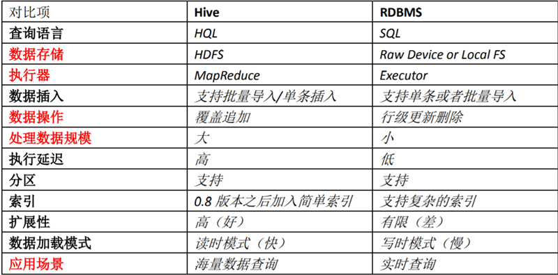
Differences between Hive and ordinary relational databases.

• Query language. Hive provides a SQL-like query language, HQL, which can be used directly by developers familiar with SQL.
• Hive is built on Hadoop, and all Hive data is stored in HDFS. The database, on the other hand, can store data on a block device or local file system.
• There is no specific data format defined in Hive, the data format can be specified by the user, who has to specify three properties: the column separator (usually spaces, \t, \x001), the row separator (\n) and the method of reading the data from the file (there are three default file formats in Hive: TextFile, SequenceFile and RCFile). As there is no conversion from the user data format to the data format defined by Hive during the loading process, Hive does not make any changes to the data itself during the loading process, but simply copies or moves the data contents to the appropriate HDFS directory. In contrast, in databases, different databases have different storage engines that define their own data formats. All data is stored according to a certain organisation, so the process of loading data into a database can be more time consuming.
• Data updates. As Hive is designed for data warehouse applications, which are more read and less written. Therefore, there is no support for rewriting or adding to data in Hive; all data is determined at load time. The data in the database is usually modified frequently, so you can add data using INSERT INTO … VALUES and modify data using UPDATE … SET.
• Hive does not do anything to the data as it loads it, not even scan it, and therefore does not index certain Keys in the data. to access a specific value in the data that meets a condition, Hive has to brute-force scan the entire data, so access latency is high. Thanks to the introduction of MapReduce, Hive can access data in parallel, so even without indexes, Hive can still be advantageous for large volumes of data. In databases, indexes are usually created for one or a few columns, so databases can be very efficient and have low latency for accessing small amounts of data with specific conditions. The high latency of accessing data dictates that Hive is not suitable for online data queries.
• Execution. most queries in Hive are executed through MapReduce provided by Hadoop. Databases usually have their own execution engines.
• Execution latency. Hive has high latency when querying data because there are no indexes and the entire table needs to be scanned. Another factor that contributes to the high execution latency of Hive is the MapReduce framework. Because MapReduce itself has high latency, there is also high latency when executing Hive queries using MapReduce. In contrast, database execution latency is low. Of course, this low latency is conditional on the size of the data being small, and Hive’s parallel computing is clearly an advantage when the data is large enough to exceed the database’s processing power.
• Scalability. Since Hive is built on Hadoop, the scalability of Hive is consistent with the scalability of Hadoop. Databases, on the other hand, have very limited scalability rows due to the strict limitations of ACID semantics. Oracle, the most advanced parallel database available, has a theoretical scalability of only about 100 machines.
• Data size. Because Hive is built on a cluster and can use MapReduce for parallel computing, it can support very large data sizes; the corresponding database can support smaller data sizes.

To be clear, Hive, as a data warehouse application tool, has 3 “no’s” compared to RDBMS (relational database).

• Can’t respond in real time like an RDBMS, Hive has a large query latency
• Can’t do transactional queries like RDBMS, Hive has no transaction mechanism
• Can’t do row-level change operations (including insert, update, delete) like RDBMS

In addition, Hive is a more “relaxed” world than RDBMS, for example.

• Hive doesn’t have a fixed-length varchar type, strings are all string
• Hive is in read-time mode, it doesn’t validate the data when it saves the table data, instead it checks the data when it reads it to set it to NULL if it doesn’t match the format

Hive’s architecture

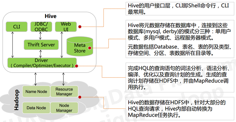
The Hive architecture consists of the following components: CLI (command line interface), JDBC/ODBC, Thrift Server, WEB GUI, metastore and Driver (Complier, Optimizer and Executor). Optimizer and Executor), these components can be divided into two main categories.

• Server-side components.
  • Driver component: this component includes Complier, Optimizer and Executor, its role is to parse the HiveQL (SQL-like) statements we write, compile and optimize them, generate an execution plan, and then call the underlying mapreduce computation framework.
  • Metastore component: metadata service component, this component stores hive’s metadata, hive’s metadata is stored in a relational database, hive supports relational databases such as derby, mysql. metadata is very important to hive, so hive supports the metastore service as a separate component, installed in a remote server cluster The metastore service can be decoupled from the hive service and the metastore service to ensure robustness of hive operation.
  • Thrift service: thrift is a software framework developed by facebook, which is used to develop scalable and cross-language services. hive integrates with this service, allowing different programming languages to call hive’s interface.
• Client-side components.
  • CLI: command line interface.
  • Thrift client: The Thrift client is not written in the architecture diagram above, but many of the client interfaces of the hive architecture are built on top of the thrift client, including the JDBC and ODBC interfaces.
  • WEB GUI: The hive client provides a way to access the services provided by hive via the web. This interface corresponds to hive’s hwi component (hive web interface) and requires the hwi service to be started before use.

Hive Data Storage

Hive’s storage structure consists of databases, tables, views, partitions and table data. Databases, tables, partitions, etc. all correspond to a directory on HDFS. All data in Hive is stored in HDFS and there is no special data storage format, as Hive is in Schema On Read mode and can support TextFile, SequenceFile, RCFile or custom formats.

Hive does not have a special format for storing data, nor does it create indexes for the data, so you can organise the tables in Hive very freely, simply by telling Hive the column and row separators in the data when you create the table, and Hive can parse the data. Secondly, all the data in Hive is stored in HDFS, which contains the following data models: Table, External Table, Partition, Bucket.

• A Table in Hive is conceptually similar to a Table in a database, in that each Table has a corresponding directory in Hive where the data is stored. For example, a table pvs has a path in HDFS: /wh/pvs, where wh is the directory of the data warehouse specified by ${hive.metastore.warehouse.dir} in hive-site.xml, and all Table data (excluding External Table) is stored in this directory. All Table data (excluding External Table) is stored in this directory.
• A Partition corresponds to a dense index of Partition columns in a database, but the way in which Partitions are organised in Hive is very different to that in a database. In Hive, a Partition in a table corresponds to a directory under the table, and all the data for the Partition is stored in the corresponding directory. For example, if the pvs table contains two Partitions, ds and city, the HDFS subdirectory corresponding to ds = 20090801, ctry = US would be: /wh/pvs/ds=20090801/ctry=US; the HDFS subdirectory corresponding to ds = 20090801, ctry = CA would be: /wh/pvs/ ds=20090801/ctry=CA
• Buckets compute hash on specified columns and slice data based on hash values, for parallelism purposes, with each Bucket corresponding to one file. The HDFS directory with hash value 0 is: /wh/pvs/ds=20090801/ctry=US/part-00000; the HDFS directory with hash value 20 is: /wh/pvs/ds=20090801/ ctry=US/part-00020
• External Table refers to data that already exists in HDFS and can be created as a Partition; it is the same as a Table in terms of metadata organization, but the actual data storage is much different.
  • The Table creation process and the data loading process (both of which can be done in the same statement), during the data loading process the actual data is moved to the data warehouse directory, after which access to the data will be done directly in the data warehouse directory. When a table is deleted, the data and metadata in the table are deleted at the same time.
  • The actual data is stored in the HDFS path specified after LOCATION and is not moved to the data warehouse directory. It is not moved to the data repository directory. When an External Table is deleted, it is only deleted.

Hive Metastore

Hive’s metastore component is a central repository for hive metadata. the metastore component consists of two parts: the metastore service and the backend data store. The backend data storage medium is a relational database, such as hive’s default embedded disk database derby, and a mysql database. the metastore service is a service component that is built on top of the backend data storage medium and can interact with the hive service. by default, the metastore service and the hive service are installed together and run in the same process. By default, the metastore service and the hive service are installed together, running in the same process. I can also strip the metastore service from the hive service, and install the metastore independently in a cluster, so that hive can call the metastore service remotely. This provides better manageability and security. Using a remote metastore service allows the metastore service and the hive service to run in separate processes, which also ensures the stability of hive and improves the efficiency of the hive service.

Hive stores metadata in the RDBMS and there are three modes to connect to the database.

• Single User Mode: This mode connects to an In-memory database Derby, typically used for Unit Tests.
• Multi User Mode: Connects to a database over the network and is the most frequently used mode.
• Remote Server Mode: Used for non-Java clients to access the meta-database. A MetaStoreServer is started on the server side and the client accesses the meta-database through the MetaStoreServer using the Thrift protocol.

Hive field types

decimal usage: Usage: decimal(11,2) represents a maximum of 11 digits, of which the last 2 are decimal and the integer part is 9; if the integer part is more than 9, the field becomes null; if the decimal part is less than 2, it is followed by 0 to make up the two digits, if the decimal part is more than two, the excess is rounded up. You can also write decimal directly without specifying the number of digits, the default is decimal(10,0) 10 integers, no decimals

Introduction to Hive SQL

Hive query statements

Hive Select syntax is almost the same as that of Mysql and other RDBMS SQL, the following syntax format is attached, no detailed explanation will be given.

SELECT Syntax and Sequence

1
2
3
4
5
6
7

SELECT [ALL | DISTINCT] select_expr, select_expr, ...
FROM table_reference
[WHERE where_condition]
[GROUP BY col_list]
[ORDER BY order_condition]
[DISTRIBUTE BY distribute_condition [SORT BY sort_condition] ]
[LIMIT number]

Multidimensional aggregation analysis grouping sets/cube/roolup

Without the multidimensional aggregation method.

1
2
3
4
5
6
7
8

SELECT NULL, NULL, NULL, COUNT(*)
FROM requests
UNION ALL
SELECT os, device, NULL, COUNT(*)
FROM requests GROUP BY os, device
UNION ALL
SELECT null, null, city, COUNT(*)
FROM requests GROUP BY city;

Using grouping sets.

1
2
3

SELECT os, device, city ,COUNT(*)
FROM requests
GROUP BY os, device, city GROUPING SETS((os, device), (city), ());

The cube will enumerate all possible combinations of the specified columns as grouping sets, while roolup will generate grouping sets in a hierarchical aggregation manner. e.g.

1
2
3
4
5
6
7

GROUP BY CUBE(a, b, c)  
--等价于以下语句。  
GROUPING SETS((a,b,c),(a,b),(a,c),(b,c),(a),(b),(c),())

GROUP BY ROLLUP(a, b, c)
--等价于以下语句。  
GROUPING SETS((a,b,c),(a,b),(a), ())

The regular method specifies SELECT field columns

It says specify, but it’s actually exclude, e.g. (num|uid)? +. + excludes the num and uid columns. Alternatively, where can be used with a regular like this: where A Rlike B, where A Regexp B.

Lateral View (one row to many rows)

Lateral View is used in conjunction with table generation functions such as Split, Explode, etc., which can split a row of data into multiple rows of data and aggregate the split data.

Suppose you have a table pageAds with two columns of data, the first column is the pageid string and the second column is the adid_list, a comma-separated collection of ad IDs. Now you need to count the number of times all the ads appear on all the pages, so you start by using Lateral View + explode to do the normal grouping and aggregation.

1

SELECT pageid, adid FROM pageAds LATERAL VIEW explode(adid_list) adTable AS adid;

Window Functions

Hive has a rich set of window functions, the most common of which is row_number() over(partition by col order col_2), which allows you to sort by a specified group of fields.

• COUNT calculates the count value.
• AVG calculates the average value.
• MAX Calculates the maximum value.
• MIN Calculates the minimum value.
• MEDIAN Calculates the median.
• STDDEV Calculates the overall standard deviation.
• STDDEV_SAMP Calculates the sample standard deviation.
• SUM Calculates the summary value.
• DENSE_RANK Calculates the continuous ranking.
• RANK Calculates jump ranking.
• LAG Takes the value of the row before the current row by offset.
• LEAD Takes the value of the row after the current row by offset.
• PERCENT_RANK Calculates the relative rank of a row in a set of data.
• ROW_NUMBER Calculates the row number.
• CLUSTER_SAMPLE Used for group sampling.
• CUME_DIST Calculates the cumulative distribution.
• NTILE Slices grouped data in order and returns the slice value.

Hive definition variables

1
2
3
4
5
6
7
8

SET aa='10';
SELECT ${hiveconf:aa};

SET hivevar:aa='10';
SELECT ${hivevar:aa};

SET hiveconf:aa='10';
SELECT ${hiveconf:aa};

CTE syntax and definition of variables

 1
 2
 3
 4
 5
 6
 7
 8
 9
10
11
12
13
14
15

with t1 as(
    select user_id
    from user
    where ...
)

@var:= select
         shop_id
       from shop
       where ...;

select *
from user_shop
where user_id in(select * from t1)
and shop_id in(select * from @var);

Hive Definition Statements (DDL)

Hive table build statement format

Method 1: Standalone statement

 1
 2
 3
 4
 5
 6
 7
 8
 9
10

CREATE [EXTERNAL] TABLE [IF NOT EXISTS] table_name
[(col_name data_type [DEFAULT value] [COMMENT col_comment], ...)]
[COMMENT table_comment]
[PARTITIONED BY (col_name data_type [COMMENT col_comment], ...)]
[CLUSTERED BY (col_name [, col_name, ...]) [SORTED BY (col_name [ASC | DESC] [, col_name [ASC | DESC] ...])] INTO number_of_buckets BUCKETS] 
[STORED BY StorageHandler] -- 仅限外部表
[WITH SERDEPROPERTIES (Options)] -- 仅限外部表
[LOCATION OSSLocation]; -- 仅限外部表
[LIFECYCLE days]
[AS select_statement]

Method 2: Copy directly from an existing table

1

CREATE TABLE [IF NOT EXISTS] table_name LIKE existing_table_name

The following is an explanation of the key declarations.

• [EXTERNAL]: declared as an external table, often declared when the table needs to be shared by multiple tools, external table deletion will not delete data, only metadata.
• col_name datatype: data_type must be strictly defined to avoid the lazy practice of using string for bigint, double, etc., otherwise the data will be wrong some day. (A colleague in the team has made this mistake)
• [if not exists]: if not specified when creating, an error will be returned if a table with the same name exists. Specify this option to ignore subsequent tables with the same name if they exist, and create them if they don’t.
• [DEFAULT value]: Specify the default value for the column, which is written to the default value when the INSERT operation does not specify the column.
• [PARTITIONED BY]: Specifies the partition field of the table. When partitioning a table using the partition field, adding a new partition, updating data within the partition and reading data from the partition do not require a full table scan, which can improve processing efficiency.
• [LIFECYCLE]: is the life cycle of the table, partitioned tables have the same life cycle as the table life cycle for each partition
• [AS select_statement]: means that data can be inserted directly with the select statement

Simple example: Create a table sale_detail to hold sales records, which uses sale_date and sale_region as partition columns.

1
2
3
4
5
6
7

create table if not exists sale_detail
(
shop_name     string,
customer_id   string,
total_price   double
)
partitioned by (sale_date string, region string);

A successfully created table can be viewed as defined by the following desc

1
2

desc <table_name>;
desc extended <table_name>; --查看外部表信息。

If you do not remember the full table name, you can look it up within the db (database) by using show tables.

1
2

use db_name;
show tables ('tb.*'); --- tb.* 为正则表达式

Hive delete table statement format

1
2

DROP TABLE [IF EXISTS] table_name;  --- 删除表
ALTER TABLE table_name DROP [IF EXISTS] PARTITION (partition_col1 = partition_col_value1,  ...); --- 删除某分区

Hive change table definition statement format

1
2
3
4
5

ALTER TABLE table_name RENAME TO table_name_new;  --- 重命名表
ALTER TABLE table_name ADD [IF NOT EXISTS] PARTITION (partition_col1 = partition_col_value1 ...);  --- 增加分区
ALTER TABLE table_name ADD COLUMNS (col_name1 type1 comment 'XXX');  --- 增加列，同时定义类型与注释
ALTER TABLE table_name CHANGE COLUMN old_col_name new_col_name column_type COMMENT column_comment;  --- 修改列名和注释
ALTER TABLE table_name SET lifecycle days;  --- 修改生命周期

Hive operation statements

Hive insert statement format.

1
2
3

INSERT OVERWRITE|INTO TABLE tablename [PARTITION (partcol1=val1...]
select_statement
FROM from_statement;

The following is an explanation of the key declarative statements.

• into|overwrite: into- appends data directly to a table or partition of a table; clears the table of existing data before inserting data into the table or partition.
• [PARTITION (partcol1=val1…]: expressions such as functions are not allowed, only constants.

About PARTITION: Specified partition inserts and dynamic partition inserts are explained here

• Output to the specified partition: Specify the partition value directly in the INSERT statement and insert the data into the specified partition.
• Output to dynamic partition: Instead of specifying the partition value directly in the INSERT statement, only the partition column name is specified. The value of the partition column is provided in the SELECT clause and the system automatically inserts the data into the corresponding partition based on the value of the partition field.

HIVE SQL Optimisation

Column Trimming

For example, if a table has five fields a,b,c,d,e, but we only need a and b, then use select a,b from table instead of select * from table

Partition Trimming

Reduce unnecessary partitioning during the query, i.e. try to specify partitions

small tables before large tables after

When writing code statements with joins, tables/subqueries with few entries should be placed before the join operator

Because the table to the left of the join operator will be loaded into memory first during the Reduce phase, loading a table with fewer entries can effectively prevent an overflow of memory (OOM). So for the same key, the smaller value is put first and the larger one is put second

Avoid using distinct as much as possible

Try to avoid using distinct for reordering, especially for large tables, which are prone to data skewing (key like in a reduce process). Use group by instead.

1
2

select distinct key from a
select key from a group by key