Open Source Distributed Query Engine - Presto

What is Presto?

Presto is Facebook’s open source MPP (Massive Parallel Processing) SQL engine, which derives its idea from a parallel database called Volcano, which proposes a model for parallel execution of SQL that is designed to be used exclusively for high-speed, real-time data analysis. Presto is a SQL computation engine, separating the computation and storage layers, which does not store data and enables access to various data sources (Storage) through the Connector SPI.

Hadoop provides a complete solution for big data storage and computation, but it uses the MapReduce computing framework, which is only suitable for offline and batch computation and cannot meet the performance requirements of fast real-time Ad-Hoc (instant analysis) query computation. However, as more and more data becomes available, a simple data query using Hive can take minutes to hours, which clearly does not meet the needs of interactive queries. Comparison with Hive.

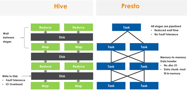
The above diagram shows the difference between MapReduce and Presto execution process. Each operation of MR either needs to write to disk or wait for the previous stage to finish before starting execution, while Presto converts SQL into multiple stages, each stage is executed by multiple tasks, and each task will be divided into multiple splits. All the tasks are allowed in parallel, and the data is executed in pipeline between stages, and the data is transferred to and from the network in the form of Memory-to-Memory, without disk io operations. This is the decisive reason why Presto’s performance is many times faster than Hive.

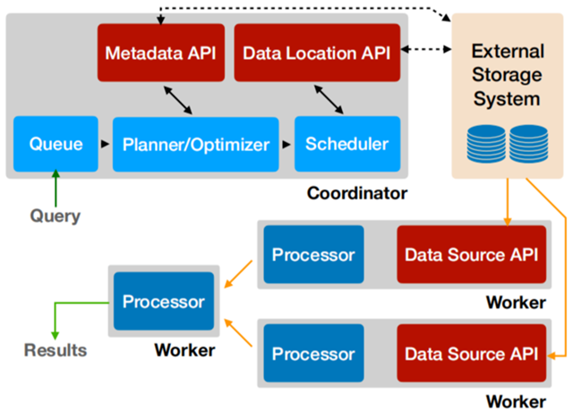
Presto follows a common Master-Slave architecture, with one Coordinator and multiple Workers, and the Coordinator is responsible for parsing SQL statements, generating execution plans, and distributing execution tasks to the Worker nodes for execution; the Worker nodes are responsible for actually executing the query tasks. Presto provides a set of Connector interfaces for reading meta information and raw data, and Presto has a variety of built-in data sources, such as Hive, MySQL, Kudu, Kafka, etc. At the same time, Presto’s extension mechanism allows customizing the Connector to enable querying of custom data sources. If a Hive Connector is configured, a Hive MetaStore service needs to be configured to provide Hive meta information to Presto, and the Worker nodes interact with HDFS through the Hive Connector to read raw data.

Advantages of Presto.

• Ad-hoc, expect query times in seconds or minutes
• 10 times faster than Hive
• Support multiple data sources, such as Hive, Kafka, MySQL, MonogoDB, Redis, JMX, etc., or you can implement your own Connector
• Client Protocol: HTTP+JSON, support various languages(Python, Ruby, PHP, Node.js Java)
• JDBC/ODBC connection support
• ANSI SQL, support for window functions, joins, aggregates, complex queries, etc.

Disadvantages of Presto.

• No fault tolerance; when a Query is distributed to multiple Workers to execute, when one Worker fails because of various reasons, then the Master will sense that the entire Query also failed, and Presto does not have a retry mechanism, so the user side needs to implement a retry mechanism.
• Memory Limitations for aggregations, huge joins; for example, multi-table joins require a lot of memory, and since Presto is a pure memory calculation, Presto does not dump the results to disk when there is not enough memory, so the query also fails, but the latest version of Presto already supports Write to disk operation.
• MPP (Massively Parallel Processing) architecture; this can not be said to be a disadvantage, because the MPP architecture is the solution to a large amount of data analysis, but its disadvantages are also very obvious, if we access the Hive data source, if one of the Worke due to load problems, data processing is very slow, then the entire query will be affected, because the upstream needs to wait for the upstream results.

Presto’s architecture

Architecture

The Presto query engine is a Master-Slave architecture, where the Coordinator is the master and the worker is the slave. A Presto cluster consists of a Coordinator node, a Discovery Server node (usually embedded in the Coordinator node), and multiple Worker nodes. Among them, the Coordinator is responsible for receiving query requests, parsing SQL statements, generating execution plans, scheduling tasks to Worker nodes for execution, and worker management; Worker nodes are work nodes, responsible for actually executing the query task Task.

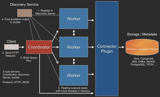
Worker node starts and registers with Discovery Server service; Coordinator obtains the Worker node from Discovery Server that can work properly.

Query execution process

The overall query process is.

• Client sends a query request using HTTP protocol.
• Discovery Server discovers the available Server through Discovery Server.
• Coordinator builds the query plan (Connector plugin provides Metadata)
• Coordinator sends a task to workers
• Worker reads data via Connector plugin
• Worker executes the task in memory (Worker is a purely in-memory compute engine)
• Worker returns the data to the Coordinator, and then Responds Client afterwards

SQL execution flow.

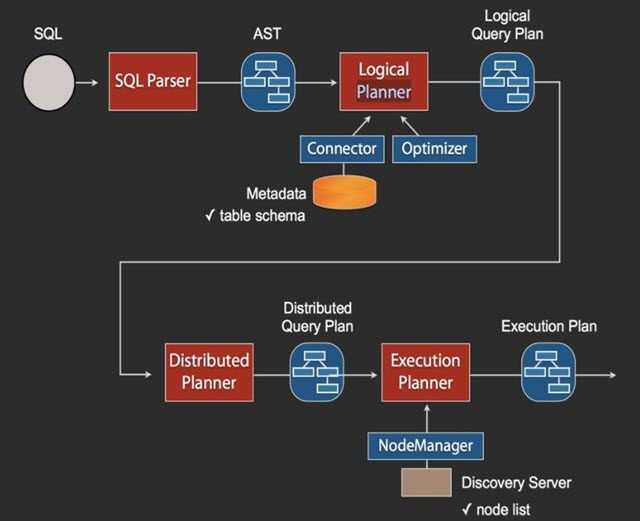
When the Coordinator receives a Query, the SQL execution process is as shown in the above figure. the SQL is parsed into AST (Abstract Syntax Tree) by Anltr3, and then the original data Metadata information is obtained through the Connector. The logical plan is generated, and then the distribution plan and execution plan are generated in turn. In the execution plan, we need to go to Discovery to get the list of available nodes, and then according to a certain policy, these plans are distributed to the specified Worker machines, which are then executed separately.

Presto contains three types of roles, coordinator, discovery, and worker. coordinator is responsible for query parsing and scheduling. discovery is responsible for cluster heartbeat and role management. worker is responsible for performing computations.

• The query submitted by presto-cli is actually an http POST request. After the query request is sent to the coordinator, it undergoes lexical and syntactic parsing to generate an abstract syntax tree that describes the execution of the query.
• The execution plan compiler, based on the abstract syntax tree, expands the structure represented by the syntax tree into a tree-like execution structure consisting of individual operations, called a logical execution plan.
• The original logical execution plan, which directly represents the operations expected by the user, may not be the best performance. At this point, the logical execution plan already includes the map-reduce operation and the transfer of intermediate computation results across machines.
• The scheduler obtains the data distribution from the data meta, constructs the split, and schedules the corresponding execution plan to the corresponding worker with the logical execution plan.
• On the worker, the logical execution plan generates the physical execution plan, and according to the logical execution plan, it generates the execution bytecode and the operator list. operator is handed over to the execution driver to complete the computation.

Abstract Syntax Tree

A tree structure generated by the syntax parser based on SQL, parsed to describe the execution process of SQL. In the following, the SQL select avg(response_size) as a , client_address from localfile.logs.http_request_log group by client_address order by a desc limit 10 is used as example to describe.

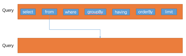
The abstract syntax tree describes the query in terms of Query, with a hierarchy representing the subqueries at different levels. Each level of query contains several key elements: select, from,where,group by,having,order by,limit. where from can be a subquery or a table.

A typical abstract syntax tree.

Generate logic execution plan

The abstract syntax tree tree, which describes the most primitive user requirements. The information described by the abstract syntax tree is not optimal in terms of execution efficiency and the execution operations are too complex. The abstract syntax tree needs to be transformed into an execution plan. The execution plan is divided into two categories, one is the logical execution plan and the other is the physical execution plan. Logical execution plans, which describe execution in a tree structure, where each node is the simplest operation. The physical execution plan, which generates bytecode based on the logical execution plan, is handed over to the driver for execution.

The process of transcription into a logical execution plan, including transcription and optimization. The abstract syntax tree is transcribed into a node tree consisting of simple operations, and then all aggregate computation nodes in the tree are transcribed into map-reduce form. And insert Exchange nodes in the middle of map-reduce nodes. Then, a series of optimizations are performed to push down some nodes that can accelerate the computation in advance and merge the nodes that can be merged.

Finally, the logical execution plan is divided into different segments (fragament) according to the Exchange nodes, which represent the execution plans of different phases. In scheduling, the execution is scheduled according to the fragment.

1
2
3
4
5

SELECT avg(response_size) as a , client_address 
FROM localfile.logs.http_request_log
GROUP BY client_address
ORDER BY a DESC
LIMIT 10

The execution logic of the above SQL.

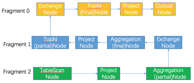
As you can see from the execution plan, the agg nodes are split into two steps, partial and final.

Scheduling execution plan to machines

Scheduling involves two issues, first, which machines a certain fragment is assigned to be executed by, and second, how the computation result of a certain fragment is output to the downstream fragment.

In scheduling, it is necessary to specify for each fragment to which machines it is assigned. In terms of scheduling, there are three types of fragment

• One type is the source type, where the original data storage location determines the scheduling machine of the fragment, how many source nodes are there? If network-topology=flat is specified in the configuration, try to select the machine where the split is located.
• Generally, only the final output node is assigned one machine, and the intermediate computation results are assigned to multiple machines. The number of allocated machines is determined by the configuration hash_partition_count. The selection of machines is random.
• One type is SINGLE type, only one machine, mainly used for aggregating results, and one machine is randomly selected.

For the output of the computation result, there are also various ways, depending on the number of machines in the downstream node.

• If there are multiple machines in the downstream node, for example, the intermediate result of group by, the hash is calculated according to the key of group by, and a downstream machine is selected according to the hash value. For non-group by calculation, it will randomly select or round robin.
• If there is only one machine in the downstream node, it will be output to this machine.

In the following figure, for example, fragment 2 is a source type fragment with three splits, so three machines are assigned. Because this layer of computation is group by aggregation, the output is computed according to the key of group by to calculate the hash and select one of the downstream machines for output.

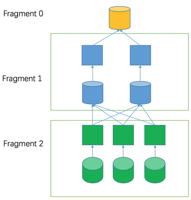
The tasks before scheduling are done in the coordinator, and after scheduling is done, the tasks are sent to the worker for execution afterwards.

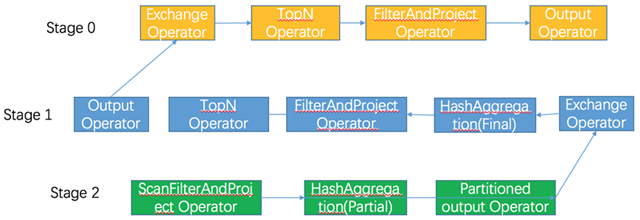
Generate physical execution plan

After the logical execution plan fragment is sent to the machine, it is transcribed into an operator list in the form of a node tree and dynamically compiled to generate bytecode according to the logical code. Dynamic generation of bytecode, mainly using the compilation principle.

• Expanding the loop
• Directly calling the right function to be used according to the type of data column to reduce branch jumping statements.

These means will make better use of the CPU pipeline.

Execution Driver

The physical execution plan constructs the generated Operator list and hands it to the Driver for execution. Exactly which data is computed is determined by the loaded Split.

Operator list processes data in a serial form, and the result of the previous operator is used as input for the next result. For operators of type source, a new copy of data is fetched with each call; for operators of type Aggregate, the output result is fetched only after all previous operators are finished. only after all previous operators are finished.

Aggregate Computation

The generated execution plans have the aggregation computation split into two steps, Map and Reduce.

There are two types of Operators for aggregation computation, AggregationOperator and HashAggregationOperator.

AggregationOperator computes all rows and updates the results to a single location; HashAggregationOperator uses the hash value of a column as the key of the hash table, and only rows with the same key will save the results together for the group by class.

Aggregation calculations are to be executed in the form of Map-Reduce.

The functions provided by the aggregation calculations have to provide four interfaces, with two inputs and two outputs, respectively:

• Accepts raw data as input.
• Accepts input from intermediate results.
• Outputs the intermediate results.
• Outputs the final result.

1+3 constitutes a Map operation 2+4 constitutes a Reduce operation.

Take Avg as an example.

• Map phase input 1,2,3,4
• Map truncated output 10,4 represents Sum and Count respectively
• Reduce input 10,4
• Reduce output final average 5

We modified the Presto system to enable Presto to provide caching functionality, which is a layer of computation added in the middle of MapReduce to accept intermediate result inputs and intermediate result outputs.

Functions

There are two types of functions, namely Scaler and Aggregate functions

• Scaler function provides data conversion processing, does not save the state, an input to produce an output.
• Aggregate function provides data aggregation processing, using existing state + input to produce new state.

Data model

Presto takes a three-tier table structure.

• catalog corresponds to a certain type of data source, such as data from hive, or data from mysql
• schema corresponds to the database in mysql
• table corresponds to a table in mysql

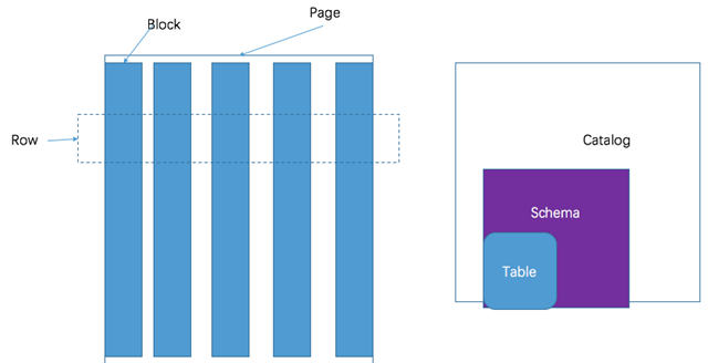
Presto’s storage units include.

• Page: A collection of multiple rows of data, containing multiple columns of data, with only logical rows provided internally, actually stored in columnar format.
• Block: a column of data, depending on the type of data, usually take a different encoding, understanding these encoding methods, help their own storage system to interface with presto.

Different types of blocks.

• array type block, applied to fixed-width types, such as int, long, double. block consists of two parts
  • boolean valueIsNull[] Indicates whether each row has a value.
  • T values[] The specific value of each row.
• Variable-width block, applied to string-like data, consists of three parts of information
  • Slice : A string with all rows of data stitched together.
  • int offsets[] : The starting cheap position of each row of data. The length of each line is equal to the starting bargain of the next line minus the starting bargain of the current line.
  • boolean valueIsNull[] : Indicates whether a row has a value. If there is a row with no value, then the cheap amount of this row is equal to the offset of the previous row.
• Fixed-width string type block, where all rows of data are stitched together into one long Slice, with each row having a fixed length.
• Dictionary block: For some columns, the distinct value is less, suitable for saving using dictionary. There are two main components.
  • dictionary, which can be any type of block (even a nested dictionary block), and each row in the block is sorted and numbered in order.
  • int ids[] indicates the number of the value in the dictionary corresponding to each row of data. When searching, first find the id of a row, then go to the dictionary to get the real value.

Plugins

Once you understand the data model of presto, you can write plugins to presto to interface to your own storage system. presto provides a set of connector interfaces to read metadata from custom storage, as well as column storage data. Let’s first look at the basic concepts of connector.

• ConnectorMetadata: Manage table metadata, table metadata, partition and other information. When processing a request, the meta information needs to be fetched in order to confirm the location of the read data. presto will pass in the filter condition in order to reduce the range of the read data. The meta information can be read from disk or cached in memory.
• ConnectorSplit: A collection of data processed by an IO Task, which is the unit of scheduling. A split can correspond to one partition, or multiple partitions.
• SplitManager : Constructs a split based on the meta of the table.
• SlsPageSource : Reads 0 or more pages from disk for the calculation engine based on the information of the split and the information of the columns to be read.

Plugins can help developers add these features.

• Dock to your own storage system.
• Add custom data types.
• Add custom processing functions.
• Custom permission control.
• Custom resource control.
• Add query event handling logic.

Presto provides a simple connector: the local file connector , which can be used as a reference for implementing your own connector, but the local file connector uses a cursor to traverse the data, i.e. a row of data, not a page. hive’s connector implements three types of connectors, parquet connector, orc connector, and rc file connector.

Memory management

Presto is an in-memory computing engine, so memory management must be fine-tuned to ensure orderly and smooth execution of queries, and partial starvation, deadlocks and other situations.

Memory pooling

Presto uses a logical memory pool to manage different types of memory requirements.

Presto divides the entire memory into three memory pools, System Pool , Reserved Pool, and General Pool.

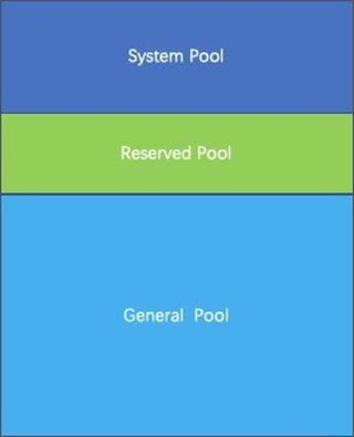
• System Pool is reserved for system use, default is 40% of the memory space reserved for system use.
• Reserved Pool and General Pool are used to allocate memory for query runtime.
• Most of the queries use the general pool. The largest query uses the Reserved Pool, so the Reserved Pool is equal to the maximum amount of space used by a query running on a machine, which is 10% by default.
• The General Pool has all the memory space except the System Pool and the General Pool.

Why memory pools are used

System Pool is used for memory used by the system, for example, data is passed between machines and buffer is maintained in the memory, which is mounted under the system name.

So, why do you need reserved area memory? And is the reserved memory exactly equal to the maximum memory used by the query on the machine?

If there is no Reserved Pool, then when there are a lot of queries and they are almost running out of memory space, one of the more memory consuming queries starts running. But then there is no more memory space for this query to run, and the query keeps hanging, waiting for available memory. But after other small-memory queries are run, new small-memory queries are added. Since small memory queries take up little memory, it is easy to find available memory. In this case, the big memory query keeps hanging until it starves.

So in order to prevent this starvation, a space must be reserved for the large memory query to run. Every second, Presto picks out a query with the largest memory footprint and allows it to use the reserved pool to avoid running out of memory for that query.

Memory Management

Presto memory management, in two parts:

• query memory management. query is divided into many tasks, each task will have a thread loop to get the state of the task, including the memory used by the task. The memory is aggregated into the memory used by the query. If the aggregated memory of a query exceeds a certain size, the query is forced to terminate.
• Machine memory management. coordinator has a thread that regularly rotates through each machine to check the current state of machine memory.

When the query memory and machine memory are aggregated, the coordinator selects a query that uses the most memory and assigns it to the Reserved Pool.

Memory management is managed by the coordinator, which makes a judgment every second to specify that a particular query can use reserved memory on all machines. So the question is, if the query is not running on a machine, isn’t the memory reserved for that machine wasted? Why not pick out the largest task on a single machine and execute it. The reason is still deadlock, if the query, which enjoys reserved memory on other machines, is executed quickly. But if it is not the largest task on a machine, it will not be run and the query will not be finished.