Network Virtualization

Network Virtualization is the process of building a virtual network with a different topology than the physical network. For example, if a company has multiple offices around the world, but wants its internal network to be one, it needs network virtualization technology.

Starting with NAT

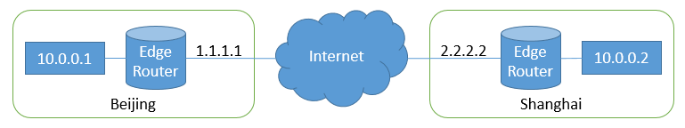
Suppose one machine in the Beijing office has an IP of 10.0.0.1 (which is an intranet IP and cannot be used on the Internet) and one machine in the Shanghai office has an IP of 10.0.0.2 and they want to communicate over the Internet. The public (Internet) IP of the Beijing office is 1.1.1.1, and the public IP of the Shanghai office is 2.2.2.2.

A simple way to do this is to change the outgoing packet source IP 10.0.0.1 to 1.1.1.1 and the destination IP 10.0.0.2 to 2.2.2.2 at the Edge Router in the Beijing office, and the incoming packet destination IP 1.1.1.1 to 10.0.0.1 and the source IP 2.2.2.2 to 10.0.0.2. The border router in the Shanghai office does a similar address translation. Thus 10.0.0.1 and 10.0.0.2 are able to communicate, completely unaware of the existence of the Internet and the address translation process. This is basic NAT (Network Address Translation).

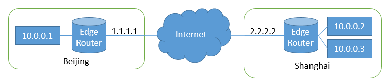
But there are serious problems with this approach. Imagine that the Shanghai office adds a machine with an intranet IP of 10.0.0.3. Regardless of what happens in the Beijing office, the border router in the Shanghai office receives a packet with a destination IP of 2.2.2.2.2, should it send it to 10.0.0.2 or 10.0.0.3? This bug seems simple enough, but it is easy for designers to overlook. When designing a network topology or network protocol, you can’t just think about how the packets go out, but also how the reply packets come in. With simple NAT, every time you add an intranet machine, you add a public IP to the border router.

We know that public IPs are valuable, and NAPT (Network Address and Port Translation) was born, and NAT in Linux is in fact NAPT. For incoming connections, the basic assumption of NAPT is that two machines sharing the same public IP will not provide the same service. For example, if 10.0.0.2 provides HTTP service and 10.0.0.3 provides HTTPS service, the border router in Shanghai office can be configured as “Destination IP is 2.2.2.2 and destination port is 80 (HTTP) to 10.0.0.2, destination port is 443 (HTTPS) to 10.0. 0.3”. This is DNAT (Destination NAT).

We know that public IPs are a valuable resource, and NAPT (Network Address and Port Translation) was born, and NAT in Linux is in fact NAPT. For incoming connections, the basic assumption of NAPT is that two machines sharing the same public IP will not provide the same service. For example, if 10.0.0.2 provides HTTP service and 10.0.0.3 provides HTTPS service, the border router in Shanghai office can be configured as “Destination IP is 2.2.2.2 and destination port is 80 (HTTP) to 10.0.0.2, destination port is 443 (HTTPS) to 10.0. 0.3”. This is DNAT (Destination NAT).

For outgoing connections, things are a little more complicated. 10.0.0.2 initiates a connection to 10.0.0.1 with a source port of 20000 and a destination port of 80. 10.0.0.3 also initiates a connection to 10.0.0.1 with a source port of 30000 and a destination port of 80. When a reply packet from the Beijing office arrives at the border router in the Shanghai office, the source port is 80 and the destination port is 20000, so if the border router does not keep the connection status, it obviously does not know to whom the packet should be forwarded. That is, the border router has to maintain a table.

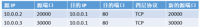
When a reply packet comes in, check the source port (80) and destination port (20000), match the first record, and know that it was sent to 10.0.0.2. Why do you need the “new source port” column? If 10.0.0.2 and 10.0.0.3 originate separate TCP connections to the same destination IP and the same destination port on the same source port, the reply packets for the two connections will be indistinguishable. In this case, the border router must assign a different source port, and the actual source port of the outgoing packet is the “new” one. Network address translation for outgoing connections is called SNAT (Source NAT).

IP-in-IP Tunneling

NAPT requires that two machines sharing a public IP cannot provide the same service, a restriction that is many times unacceptable. For example, we often need SSH or remote desktop to each machine. Tunneling technology was born. The simplest Layer 3 tunneling technology is IP-in-IP.

As shown above, the original IP packet is in black on a white background, and the header is added in white on a blue background. This header is usually added (encap) on the sender’s border router. The encapsulated header is first a Link Layer header, then a Network Layer header, and the entire packet is a legitimate IP packet that can be routed over the Internet. When the receiving border router receives this packet, it sees the IP-in-IP flag in the added header (IP protocol number = 0x04, not shown in the figure), and knows that it is a packet of IP-in-IP tunnel; it also sees that the public DIP is itself, and knows that it is time to decap. After the decap, the original packet (Private SIP, Private DIP) is revealed and then routed to the corresponding machine on the intranet.

IP-in-IP Tunneling is not enough.

1. If you try to use IP-in-IP tunneling to build a LAN with the same network address and subnet mask at both ends of the tunnel, and do not configure ARP table on the client, you will find that the clients (not the routers at both ends of the tunnel) cannot ping each other. IP-in-IP tunnel can only pass IPv4 packets, not ARP packets. (IPv4 and ARP are different three-layer protocols.) Therefore, the ARP table must be configured manually on the client, or the router can answer it for the client, which makes network configuration more difficult.

2. In a data center, there is often more than one client. For example, if two clients have both created virtual networks with intranet IPs of 10.0.0.1, if they share the same public IP when sending to the Internet, there is no way to tell which client to send an incoming IP-in-IP packet to.

3. If you want to do load balancing, you usually do hash on the packet header five-tuple (source IP, destination IP, quad protocol, source port, destination port), and select the target machine according to the hash value, so as to ensure that packets of the same connection are always sent to the same machine. If an ordinary network device doing load balancing receives an IP-in-IP packet, if it does not recognize the IP-in-IP protocol, it cannot resolve the four-layer protocol and port number, and can only do hash based on Public SIP and Public DIP, which are generally the same, then only the source IP is a variable, and the uniformity of hash is hard to guarantee. The first problem indicates that the packet being packaged (encap) is not necessarily an IP packet. The second problem indicates that additional identification information may need to be added. The third problem is that the packet headers that are added are not necessarily IP packet headers. This is the reason why network virtualization technologies are blossoming instead of one size fits all.

Classification of network virtualization technologies

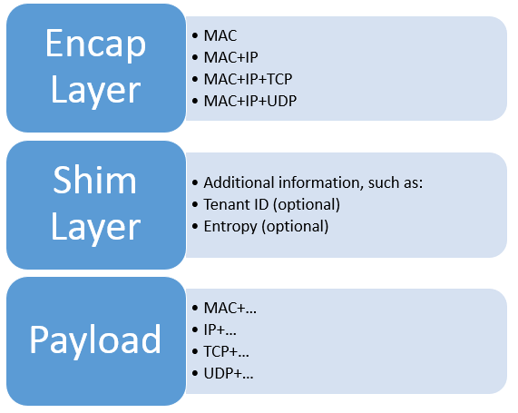
When looking at a network virtualization technology, the main thing to look at is the format of the packets in the tunnel.

• The outermost layer is the encapsulation layer, which must be MAC because it needs to be transmitted in the network and must be a legitimate layer 2 packet. when we say that the encapsulation layer is N layers, we mean that 2 … N layers of encapsulation packet headers are added and removed.
• The middle one is the optional shim layer, which contains some additional information and flag bits, such as Tenant IDs to identify different clients’ virtual networks, and Entropy to improve hash homogeneity.
• The inner layer is the actual packet sent by the client, which determines how the virtual network looks like to the client. For example, if the inner layer of an IP-in-IP tunnel is IPv4 packets, the virtual network will appear to the client as an IPv4 network running TCP, UDP, ICMP, or any other four-layer protocol. When we say that the virtual network is Layer N, we mean that the packets sent by the client at Layer 2 . N-1 layers will not be transmitted (these layers may affect the encapsulation layer, i.e. which tunnel to enter). Virtual networks are not better the lower the layer (the closer to the physical layer), because the lower the layer the harder the protocol is to optimize, as we will see later.

A simple classification of common network virtualization technologies (I include some tunneling technologies in the category of network virtualization technologies) can be made based on the format of the packets in the tunnel: (PPP and MAC are Layer 2 protocols, IP is a Layer 3 protocol, and TCP and UDP are Layer 4 protocols as described below).

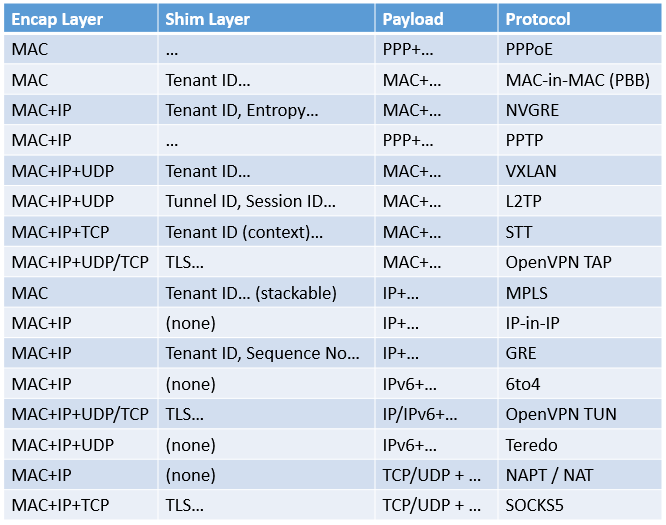
It follows that there are corresponding protocols for almost every reasonable combination of Encap Layer and Payload. Therefore, the statement that some people “add a Layer 2 header to GRE and you can …… it” is meaningless; once Encap Layer and Payload change, it is some other protocol. Here are some examples of protocols that exist at different levels, i.e., what problems it solves.

GRE vs. IP-in-IP

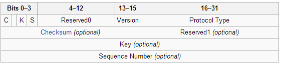
The GRE (Generic Routing Encapsulation) protocol adds an intermediate layer (shim layer) to the IP-in-IP protocol, including a 32-bit GRE Key (Tenant ID or Entropy) and sequence number information. The GRE Key solves the second problem of the IP-in-IP tunnel by allowing different clients to share the same physical network and set of physical machines, which is important in a data center.

NVGRE vs. GRE

The GRE virtual network is an IP network, which means that IPv6 and ARP packets can not be transmitted in the GRE tunnel. IPv6 is easier to solve, just change the Protocol Type in the GRE header. The ARP request packet is a broadcast packet: “Who has 192.168.0.1? Tell 00:00:00:00:00:01”, which reflects a fundamental difference between Layer 2 and Layer 3 networks: Layer 2 networks support the Broadcast Domain. Broadcast Domain. VLANs are a common way to implement a broadcast domain.

Of course, IP also supports broadcast, but packets sent to a Layer 3 broadcast address (such as 192.168.0.255) are still sent to a Layer 2 broadcast address (ff:ff:ff:ff:ff:ff:ff), which is achieved through the Layer 2 broadcast mechanism. It’s not impossible to make the ARP protocol work in GRE tunnels if we have to, it’s just that people don’t generally do it.

In order to support all existing and possible future Layer 3 protocols, and to support broadcast domains, it is necessary that the client’s virtual network be a Layer 2 network. NVGRE and VXLAN are the two best known Layer 2 network virtualization protocols.

NVGRE (Network Virtualization GRE) has only two essential changes over GRE.

• The inner Payload is a Layer 2 Ethernet frame instead of a Layer 3 IP packet. Note that the FCS (Frame Check Sequence) at the end of the inner Ethernet frame is removed because the encapsulation layer already has a checksum, and calculating the checksum would increase the system load (if the CPU is allowed to calculate it).
• The GRE key of the middle layer is split into two parts, the first 24 bits as Tenant ID and the last 8 bits as Entropy. Why use GRE when you have NVGRE? Historical and political reasons aside, the lower the level of the virtual network, the less likely it is to be optimized.
• If the virtual network is layer 2, since MAC addresses are generally very fragmented, only one forwarding rule can be inserted for each host, and the network size is the problem. If the virtual network is Layer 3, IP addresses can be assigned based on the network topology so that the IP addresses of hosts close to each other on the network are also in the same subnet (which is exactly what the Internet does), so that only the network address and subnet mask prefix matches on the router based on the subnet can reduce a large number of forwarding rules.
• If the virtual network is layer 2, packets such as ARP broadcasts are broadcast to the entire virtual network, so layer 2 networks (what we often call LANs) generally cannot be too large. If the virtual network is Layer 3, this problem does not exist because IP addresses are assigned on a cascading basis.
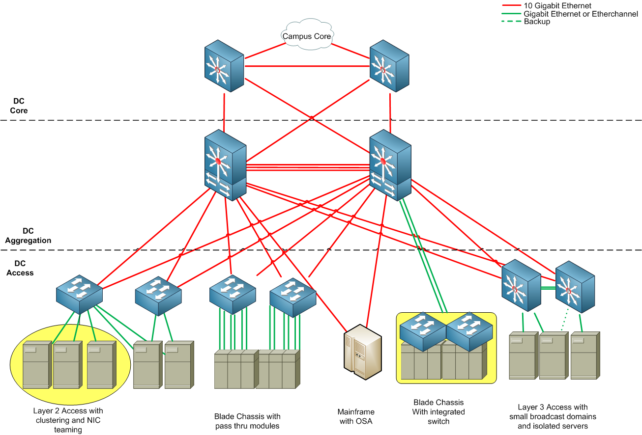
• If the virtual network is Layer 2, the switch relies on the spanning tree protocol to avoid loops. If the virtual network is Layer 3, multiple paths between routers can be leveraged to increase bandwidth and redundancy. The network topology of a data center is typically shown in the following diagram (image source)

Virtual networks are generally not called “virtual networks” if they are at a higher level and do not include a network layer in the payload, but they still fall under the category of tunneling technology. SOCKS5 is one such protocol where the payload is TCP or UDP. It has more configuration flexibility than IP-based tunneling, for example, you can specify port 80 (HTTP protocol) for one tunnel and port 443 (HTTPS protocol) for another. ssh’s -L (local forwarding) and -D (dynamic forwarding) parameters are used in the SOCKS5 protocol. the downside of SOCKS5 is that it does not support arbitrary Layer 3 protocols, such as ICMP (SOCKS4 does not even support UDP, so DNS is a bit tricky to handle).

VXLAN vs. NVGRE

NVGRE has an 8-bit entropy field, but if the network device doing load balancing does not know NVGRE protocol, it still does hash based on the five-tuple of “source IP, destination IP, quad protocol, source port, destination port”, the entropy is still not useful.

The solution for VXLAN (Virtual Extensible LAN) is to add a UDP layer to the encapsulation layer in addition to MAC and IP layers, and use the UDP source port number as the entropy and the UDP destination port number as the VXLAN protocol identity. This way, the load balancing device does not need to know the VXLAN protocol, it just needs to do hash of the packet according to the normal UDP quintet.

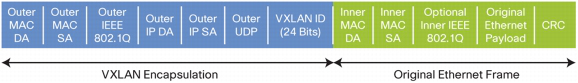
Above: Packet format after VXLAN encapsulation (image source)

The VXLAN mezzanine is slightly simpler than the GRE mezzanine, still using 24 bits as the Tenant ID and no Entropy bits. The network device or OS virtualization layer that adds the packet header typically makes a copy of the source port of the inner payload and uses it as the UDP source port for the encapsulation layer. Since the OS that initiates the connection chooses the source port number, it is generally incremental or random, and the hash algorithm inside the network device is generally XOR, so the hash uniformity is generally better.

STT vs. VXLAN

STT (Stateless Transport Tunneling) is a new network virtualization protocol that was proposed in 2012 and is still in draft form; STT, compared to VXLAN, at first glance appears to be just replacing UDP with TCP, but in fact, if you catch packets on the network that have been packetized by STT and VXLAN, they are very different.

Why does STT use TCP? In fact, STT only borrows the shell of TCP and does not use the state machine of TCP at all, not to mention the acknowledgement, retransmission and congestion control mechanisms. LSO enables the sender to generate TCP packets of up to 64KB (or even longer), and the NIC hardware to split the TCP payload part of the large packet, copy the MAC, IP, and TCP packet headers, and form a small packet (e.g., 1518 bytes for Ethernet, or 9K bytes with Jumbo Frame enabled) that can be sent out at Layer 2. The LRO allows the receiver to combine several small packets of the same TCP connection into one large packet and then generate a NIC interrupt to send to the operating system.

As shown in the figure below, the STT Frame Header (middle layer) and the MAC header, IP header, and TCP-like header (encapsulation layer) are added to the Payload before it is sent out. The NIC’s LSO mechanism will break the TCP packet into smaller pieces, copy the encapsulation layer and add it to the front of each piece before sending it out.

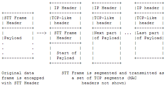
We know that user-kernel switching and NIC interrupts consume CPU time, and that the performance of network programs (e.g., firewalls, intrusion detection systems) is often measured in pps (packet per second) rather than bps (bit per second). Then when transmitting large amounts of data, the load on the system can be reduced if the packets can be larger.

The biggest problem with STT is that it is not easy to implement a policy for a particular client (tenant ID) on a network device. As shown above, for a large packet, only the first packet has an STT Frame Header in the header, while subsequent packets have no information that identifies the customer. This is not possible if I want to restrict a customer’s traffic from the Hong Kong data center to the Chicago data center to no more than 1Gbps. With other network virtualization protocols, this policy can be configured on the border router since each packet contains information that identifies the customer (of course the border router needs to be aware of this protocol).

Conclusion

This paper introduces a wide variety of network virtualization technologies using protocols such as IP-in-IP, GRE, NVGRE, VXLAN, and STT as examples. When learning a network virtualization technology, you should first figure out its encapsulation level, the level of the virtual network and the information contained in the middle layer, and compare it with other similar protocols, then look at details such as flag bits, QoS, encryption, etc. When choosing a network virtualization technology, you also need to consider the operating system and network equipment based on the level of support and the size, topology, and traffic characteristics of the customer’s network.

Reference

• https://ring0.me/2014/02/network-virtualization-techniques/
• https://www.ibm.com/developerworks/cn/linux/1310_xiawc_networkdevice/
• http://ifeanyi.co/posts/linux-namespaces-part-1/
• https://blog.scottlowe.org/2013/09/04/introducing-linux-network-namespaces/
• http://www.opencloudblog.com/?p=66

Reference https://houmin.cc/posts/f07e2cff/