Principle and Implementation of LSM-Tree and LevelDB

LSM-Tree is a data structure for write many read few application scenarios, which is adopted by powerful NoSQL databases such as Hbase and RocksDB as the underlying file organization method. In this paper, we will introduce the design idea of LSM-Tree, and analyze how LevelDB using LSM-Tree is implemented and optimized for performance.

Before understanding LSM-Tree, the storage systems I have studied, such as MySQL and etcd, are all oriented towards read-more-write-less scenarios, and most of them use B-Tree and its variants as the underlying data structure. LSM-Tree solves the problem of another application scenario - write more read less. In the scenario of storing and retrieving massive data in billions, we usually choose powerful NoSQL databases, such as Hbase, RocksDB, etc., whose file organization is modeled after LSM-Tree.

LSM-Tree

LSM-Tree, known as Log Structured Merge Tree, is a hierarchical, ordered, disk-oriented data structure, whose core idea is to leverage the fact that the sequential write performance of disk is much higher than the random write performance, converting bulk random writes into one-time sequential writes.

When we buy a disk, we are actually paying the selling price for two things: the disk capacity and the disk I/O capability. For any type of application, one of these will usually be the limiting factor. If we find that the disk spinner is fully used when adding data, but the disk has space left over, this means that the I/O capacity is a performance bottleneck for the program.

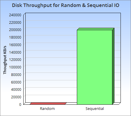
Image from Log Structured Merge Trees

As you can see visually from the graph above, sequential access to disk is at least three orders of magnitude faster than random I/O, and even sequential access to disk is faster than random access to main memory. This means that sequential access is well worth exploring and designing to avoid random I/O operations as much as possible.

The LSM-Tree is designed and optimized around this principle by eliminating random update operations to optimize write performance and provide a low-cost indexing mechanism for files with high update frequency over time, reducing query overhead.

Two-Component LSM-Tree

The LSM-Tree can be composed of two or more tree-like data structure components, and in this subsection we start with the simpler two-component case.

The above figure is modified from the LSM-Tree paper: Figure 2.1. Schematic picture of an LSM-tree of two components

The Two-Component LSM-Tree has a C0 component in memory, which can be a structure such as AVL or SkipList, and all writes are first written to C0. There is a C1 component on disk, and when the size of the C0 component reaches a threshold, a Rolling Merge is performed to merge the in-memory contents into C1. The flow of the write operation of the two-component LSM-Tree is as follows.

1. when there is a write operation, the data is first appended and written to the log file for recovery if necessary.
2. the data is then written to the C0 component located in memory, keeping the Key in order through some data structure.
3. the data in memory is flushed to disk at regular intervals or at a fixed size, and update operations are only written to memory and do not update existing files on disk.
4. as more and more write operations are performed, more and more files are accumulated on the disk, which are not writable but ordered, so we regularly perform a merge (Compaction) operation on the files to eliminate redundant data and reduce the number of files.

Similar to normal log writing, this data structure is written in an Append mode, with no deletions or modifications. Updating data that causes changes in index values is tedious and time-consuming for any application, but such updates can be easily solved by LSM-Tree by treating the update operation as a delete operation plus an insert operation.

The C1 component is optimized for sequential disk access and can be a B-Tree type data structure (SSTable implementation in LevelDB), where all nodes are 100% populated and all single-page nodes under the root node are packed onto consecutive Multi-Page Blocks for efficient disk utilization. Multi-Page Block I/O is used for Rolling Merge and long interval retrieval, which effectively reduces disk spiral arm movement, while Single-Page I/O is used for matching lookups to minimize cache size. Usually the root node has only one single-page, while the other nodes use 256KB Multi-Page Blocks.

In a two-component LSM-Tree, as long as the C0 component is large enough, then there is a batch processing effect. For example, if the size of a data record is 16 Bytes, there will be 250 records in a 4KB node; if the C0 component is 1/25 the size of C1, then for each new C1 node with 250 records resulting from a merge operation, there will be 10 new records merged from C0. This means that the user’s newly written data is temporarily stored in C0 in memory and then written to disk in a batch delay, which is equivalent to merging the user’s previous 10 writes into a single write. Obviously, the LSM-Tree is more efficient than a B-Tree structure because it only requires a single random write to write multiple pieces of data, and the Rolling Merge process is the key to this.

Rolling Merge

The Rolling Merge process of a two-component LSM-Tree can be likened to a cursor with a certain step length cyclically traversing the key-value pairs of C0 and C1, continuously taking data from C0 and putting it into C1 on disk.

The cursor has a logical location on both the leaf and index nodes of the C1 tree, and at each level, all the Multi-Page Blocks that are participating in the merge will be divided into two types: Emptying Blocks where the internal records are being moved out, but there is still some data that the cursor has not reached, and Filling Blocks that store the the result of the merge. Similarly, the cursor defines Emptying Node and Filling Node, both of which are cached in memory. To allow concurrent access, each Block at the hierarchy level contains an integer number of nodes, so that during the reorganization and merging of the executing nodes, access to the internal records of these nodes will be blocked, but other nodes in the same Block will still be accessible.

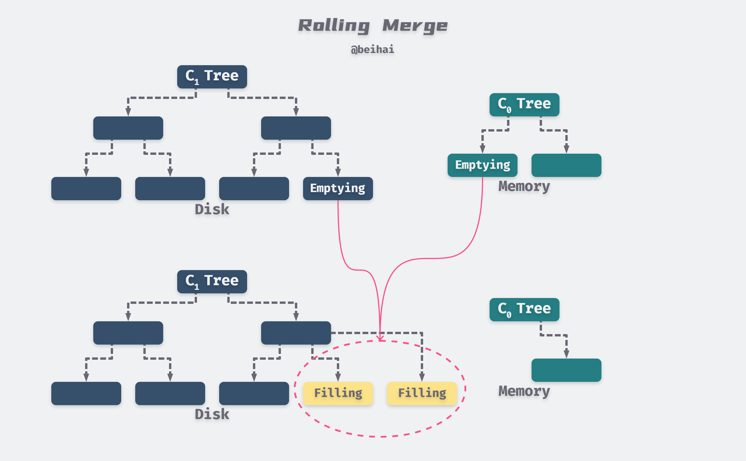
The above figure is modified from the LSM-Tree paper: Figure 2.2. Conceptual picture of rolling merge steps

The merged new Blocks are written to a new disk location so that the old Blocks are not overwritten and data recovery can still be performed after a crash. At the same time, new index information needs to be created in the index node and a log record needs to be generated for the recovery. Old Blocks that may be needed in the recovery process are not deleted for the time being, and can only be declared invalid when subsequent writes provide sufficient information.

The parent directory nodes in C1 are also cached in memory and updated in real time to reflect changes in the leaf nodes, while the parent nodes remain in memory for a period of time to minimize I/O. When the merge step is complete, the old leaf nodes in C1 become invalid and are subsequently removed from the C1 directory structure. To reduce data recovery time after a crash, the merge process requires a periodic checkpoint to force the cached information to be written to disk.

To make the LSM read relatively fast, it is important to manage the number of files, so we have to merge and compress the files. In LevelDB, the merged large files will go to the next Level.

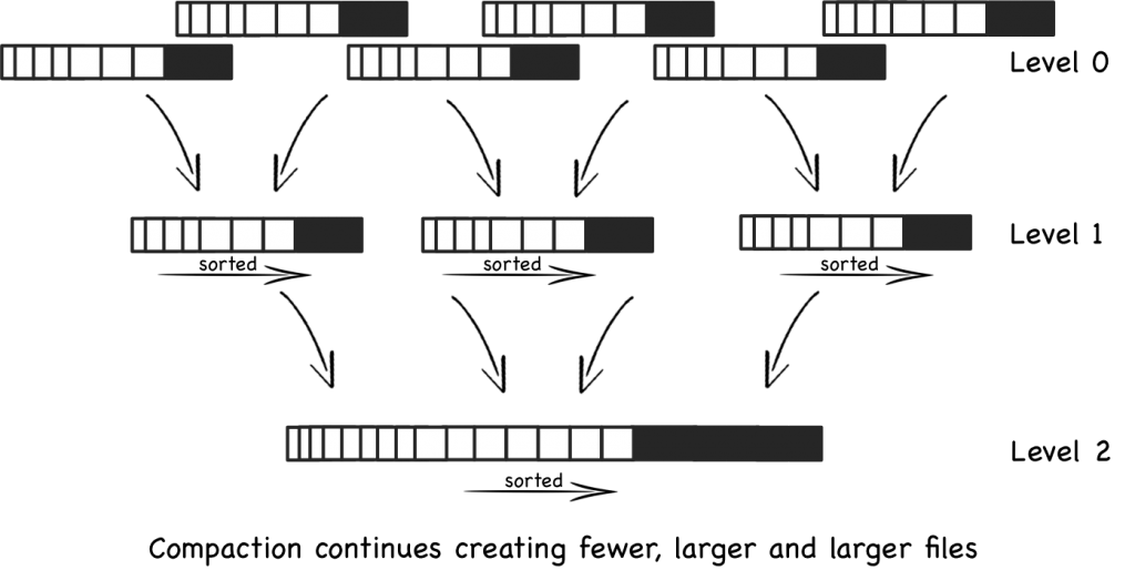
Image source: wikipedia: Log-structured merge-tree

For example, we have 10 data in each file in Level-0, and every 5 Level-0 files are merged into 1 Level1 file, and there are 50 data in each single Level1 file (which may be slightly less). And every 5 Level1 files are merged into 1 Level2 file, and the process continues to create larger and larger files, and the older the data the higher the Level level will be.

Since the files are sorted, the process of merging files is very fast, but the higher the level, the slower the data is queried. In the worst case, we need to search all files individually to read the results.

Data Reading

When performing an exact match query or a range query on the LSM-Tree, it first goes to C0 to find the desired value, and if it is not found in C0, it then goes to C1. This means that there is some additional CPU overhead compared to the B-Tree, since it now needs to go to both directories to search. While each file is kept sorted, it is possible to determine if a search is needed by comparing the max/min key-value pairs for that file. However, as the number of files increases and each file needs to be checked, reading still becomes slower and slower.

As a result, LSM-Tree is slower to read than other data structures. But we can use some indexing tricks to optimize it. LevelDB will keep block index at the end of each file to speed up the query, which is better than direct binary search because it allows to use variable-length fields and is more suitable for compressing data. The details will be described in the SSTable subsection.

We can also perform some optimizations for deletion operations to update indexes efficiently. For example, through the Predicate Deletion process, a bulk delete operation can be performed by simply declaring an assertion. For example, deleting all index values with a timestamp of 20 days ago can be achieved by directly discarding the records located in the C1 component when they are loaded into memory through the normal data merge process.

In addition, the concurrent access method for the LSM-Tree must resolve three types of physical conflicts, taking into account the following factors.

• Query operations cannot simultaneously access the node contents of a disk component being modified by another process’ Rolling Merge.
• query and insert operations against a C0 component also cannot access the same part of the tree at the same time as the Rolling Merge in progress.
• In a multi-component LSM-Tree, the Rolling Merge cursor from Ci-1 to Ci sometimes needs to leapfrog the Rolling Merge cursor from Ci to Ci+1, because the rate at which data is moved out of Ci-1 >= the rate at which it is moved out of Ci, which means that the cursor associated with Ci-1 has a faster cycle time. Therefore, in any case, the concurrent access mechanism used must allow this interleaving to occur, and not force the thread moving data into Ci to block after the thread moving data out of Ci at the rendezvous point.

Multi-Component LSM-Tree

In order to keep the size of C0 within the threshold, this requires that Rolling Merge must merge data into C1 at a rate no slower than the user’s write rate, where different sizes of C0 can have different results on overall performance.

• C0 very small: At this point, a single data insertion will make C0 full, thus triggering Rolling Merge, and in the worst case, each insertion of C0 will result in all leaf nodes of C1 being read into memory and written back to disk, with very high I/O overhead.
• C0 Very Large: There is basically no I/O overhead at this point, but it requires a lot of memory space and is not easy to perform data recovery.

The paper The Log-Structured Merge-Tree (LSM-Tree) spends a considerable amount of time on the relationship between memory capacity cost and disk I/O cost, which I will not elaborate on here, but we need to find a balance between disk I/O cost and memory capacity cost. According to the The Five-Minute Rule principle, this value depends on the performance and price of the current hardware.

In order to further reduce the overhead balance of the two-component LSM-Tree, the multi-component LSM-Tree introduces a new set of Components between C0 and C1 with sizes in between, growing step by step, so that C0 does not have to Rolling Merge with C1 each time, but first merges with the middle component, and then does Rolling Merge with C1 when the middle component reaches its size limit. This reduces the memory overhead of C0 and reduces the disk I/O overhead at the same time. This is somewhat similar to our multi-level cache structure.

In order to further reduce the overhead balance of the two-component LSM-Tree, the multi-component LSM-Tree introduces a new set of Components between C0 and C1 with sizes in between, growing step by step, so that C0 does not have to Rolling Merge with C1 each time, but first merges with the middle component, and then does Rolling Merge with C1 when the middle component reaches its size limit. This reduces the memory overhead of C0 and reduces the disk I/O overhead at the same time. This is somewhat similar to our multi-level cache structure.

Summary

The idea of LSM-Tree implementation is not quite the same as the measures taken by conventional storage systems. It converts random writes into sequential writes to try to maintain the write performance advantage of log-based databases and provide relatively good read performance. LSM-Tree is better than B-Tree and Hash in a large number of write scenarios due to two reasons.

1. Batch Write: Due to the delayed write, LSM-Tree can write multiple data to C1 in one I/O batch during the Rolling Merge process, and then the multiple data are shared equally between this I/O, reducing the I/O overhead on disk.
2. Multi-Page Block: The batch write of LSM-Tree can effectively use Multi-Page Block to read multiple consecutive data pages from C1 and merge them with C0 at one time during Rolling Merge, and then write back these consecutive pages to C1 at one time, so that only a single I/O is required to finish reading and writing multiple This allows multiple pages to be read and written in a single I/O.

The original paper of LSM-Tree is rather obscure, and it is only after the implementation of the source code of LevelDB that I can understand the author’s intention more clearly.

LevelDB

LevelDB is a standalone implementation of the key-value storage system described in the Bigtable paper “Bigtable: A Distributed Storage System for Structured Data”. It provides a high-speed key-value storage system and highly replicates the description in the paper, and many LSM-Tree implementations today refer to LevelDB.

Before introducing LevelDB, we need to understand a few basic data structures of the internal implementation. In order to compress the space occupied by data, LevelDB designs variable-length integer encoding, in which varint32 format occupies a maximum of 5 bytes, varint64 format occupies a maximum of 10 bytes, and the document Protocol Buffers Encoding : varints has a more detailed description of the format. Although the maximum number of bytes has increased, in most cases it is less than 4 bytes, reducing storage space overall. It also implements Slice, a wrapper type for strings, which reduces the data assignment overhead by referencing character arrays and provides C/C++ type character conversion.

1
2
3
4
5

class LEVELDB_EXPORT Slice {
  private:
  const char* data_; // Data Pointer
  size_t size_;      // Data Length
};

Similar to BlotDB, which I analyzed before, LevelDB is not a full-featured database, but a storage engine implemented in C++ programming language, providing a series of interfaces for external calling programs.

1
2
3
4
5

// Implementations of the DB interface
Status Put(const WriteOptions&, const Slice& key, const Slice& value) override;
Status Delete(const WriteOptions&, const Slice& key) override;
Status Write(const WriteOptions& options, WriteBatch* updates) override;
Status Get(const ReadOptions& options, const Slice& key, std::string* value) override;

The API is called in a similar way, so we will focus on the specific implementation ideas.

WriteBatch

Tracing the source code, we can see that the Put and Delete interfaces for key-value pairs are packaged into WriteBatch for batch processing, and finally the write() function is called to write to the MemTable in memory.

 1
 2
 3
 4
 5
 6
 7
 8
 9
10
11

Status DB::Put(const WriteOptions& opt, const Slice& key, const Slice& value) {
  WriteBatch batch;
  batch.Put(key, value);
  return Write(opt, &batch);
}

Status DB::Delete(const WriteOptions& opt, const Slice& key) {
  WriteBatch batch;
  batch.Delete(key);
  return Write(opt, &batch);
}

WriteBatch contains only a private std::string type string rep_, to which all modify and delete operations are added directly, and which provides the MemTable iteration interface. It contains a 12-byte Header, where the first 8-byte is the sequence of the first write operation in the WriteBatch, and the next 4-byte is the number of write operations count. Immediately after the Header is the Record array that holds the key-value pairs, each of which is formatted as a Record record inside the WriteBatch, containing the write operation type and key-value pair data.

Note: The type of the Put operation is kTypeValue and the type of the Delete operation is kTypeDeletion.

Here are some more details about constructing Record records. The Put operation writes the complete key-value pair data, while the Delete operation writes only one Key, and when querying and merging data, if you encounter a data record with operation type kTypeDeletion, you only need to discard it. This reduces the memory space occupied and speeds up the execution.

Both the key and value are written through the PutLengthPrefixedSlice() function, which writes the length of the string first, then the content of the string, and the size field can be used to quickly locate the next key-value pair.

1
2
3
4

void PutLengthPrefixedSlice(std::string* dst, const Slice& value) {
  PutVarint32(dst, value.size());
  dst->append(value.data(), value.size());
}

The iterative function Iterate() uses a while loop to sequentially transfer the write operations stored in the string to the MemTable for execution, the following code removes some unimportant check steps, and the core process is not difficult to understand, just remove the Header loop to take values.

 1
 2
 3
 4
 5
 6
 7
 8
 9
10
11
12
13
14
15
16
17
18
19
20
21
22
23
24
25
26
27
28

Status WriteBatch::Iterate(Handler* handler) const {
  Slice input(rep_);
  input.remove_prefix(kHeader);
  Slice key, value;
  while (!input.empty()) {
    char tag = input[0];
    input.remove_prefix(1);
    switch (tag) {
      case kTypeValue:
        if (GetLengthPrefixedSlice(&input, &key) &&
            GetLengthPrefixedSlice(&input, &value)) {
          handler->Put(key, value);
        } else {
          return Status::Corruption("bad WriteBatch Put");
        }
        break;
      case kTypeDeletion:
        if (GetLengthPrefixedSlice(&input, &key)) {
          handler->Delete(key);
        } else {
          return Status::Corruption("bad WriteBatch Delete");
        }
        break;
      default:
        return Status::Corruption("unknown WriteBatch tag");
    }
  }
}

WriteBatch defines a friend class WriteBatchInternal, and operations on the private string rep_ are implemented by this friend class, which shields implementation details for external callers and ensures data security.

Pre-write log

LevelDB write operations will eventually call the DBImpl::Write() function, the core part of this function will first append the data in WriteBatch to the pre-written log log_ and then write it to MemTable.

1
2
3
4
5
6
7
8

{
    mutex_.Unlock();
    status = log_->AddRecord(WriteBatchInternal::Contents(write_batch)); // Add to WAL
    if (status.ok()) {
        status = WriteBatchInternal::InsertInto(write_batch, mem_);  // Write to MemTable
    }
    mutex_.Lock();
}

In this section we first analyze the implementation of pre-written logs. WAL only provides an external AddRecord() interface to add data, which adds one Record each time it is called. Each record is composed of the following structure.

In order to improve the reading speed of logs, LevelDB introduces the concept of Block, and will read and write files one by one according to Block, the default Block size is kBlockSize = 32KB. The end of log file may contain an incomplete block, a record will never start in the last 6 bytes, because checksum, length, type need 7 bytes in total, the remaining 6 bytes are not big enough. The remaining bytes form a trailer, which is filled with zeros and must be skipped when reading.

Note: If there are exactly 7 bytes left in the current block and a new non-zero length record is added, Leveldb will fill the last 7 bytes of the block with a FIRST record and write all the user data in the later block afterwards.

To accommodate extra-long records, each record may have the following types.

1
2
3
4
5
6
7

enum RecordType {
  kZeroType = 0,    // Reserved, indicating pre-allocated files
  kFullType = 1,
  kFirstType = 2,
  kMiddleType = 3,
  kLastType = 4
};

FULL record means a complete user record is stored in the current Block, and FIRST, MIDDLE, and LAST are used to indicate that the user record is divided into multiple segments; FIRST is the first segment of the user record, LAST is the last segment of the record, and MIDDLE is the middle segment of all user data.

If we have a user data of length 98277 Bytes, then it will be divided into three segments: the first segment takes up the rest of the first block, the second segment takes up the entire second block, and the third segment takes up the first part of the third block. This will leave a 6-byte space in the third block, which is left blank as a trailer, and the records that follow will be stored from the fourth block onwards.

This record format has several advantages, one is that we do not need extra buffers for large records, and the other is that if there is an error in the reading process, we can jump directly to the next Block, which is more convenient to delimit data boundaries.

MemTable

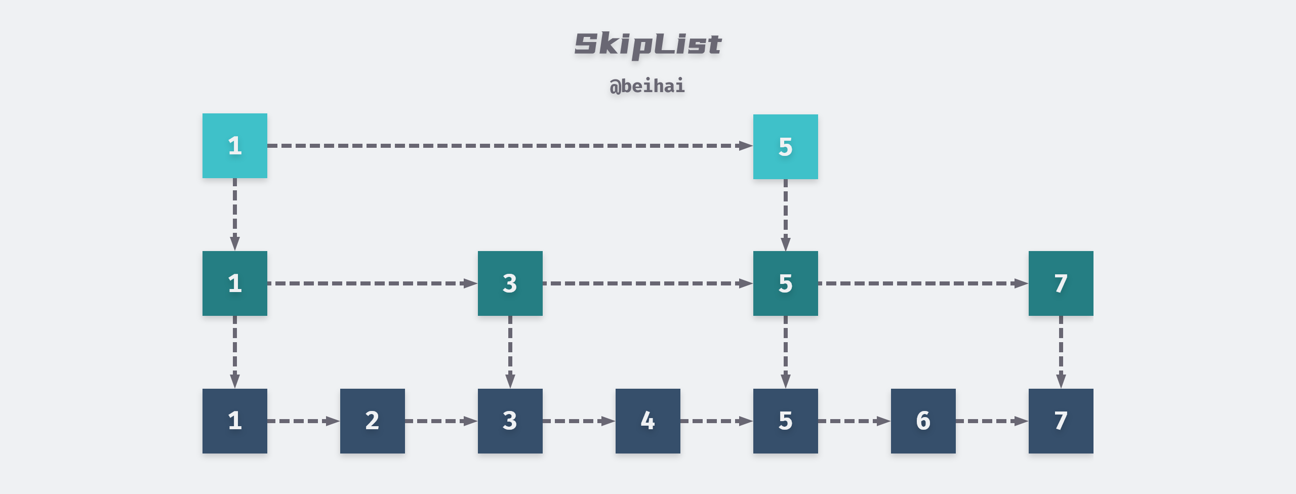
MemTable is an in-memory component of LevelDB, but it is just an interface class that wraps the API of Skip list, so the key-value pairs in MemTable are stored in an orderly way according to the Key size.

MemTable provides MemTable::Add and MemTable::Get interfaces externally, and we can see in the WriteBatch implementation that the MemTable::Add interface is called in the end, whether inserting or deleting data.

1
2
3
4
5
6
7
8

  void Put(const Slice& key, const Slice& value) override {
    mem_->Add(sequence_, kTypeValue, key, value);
    sequence_++;
  }
  void Delete(const Slice& key) override {
    mem_->Add(sequence_, kTypeDeletion, key, Slice());
    sequence_++;
  }

The Add interface encapsulates the key into a structure ParsedInternalKey and serializes it into a string. The structure ParsedInternalKey contains three fields, the sequence mentioned above is a uint64 type sequence number, but it is only 56 bits long at most, so that it can be combined with the 8-bit length ValueType to form an 8-byte composite sequence number and added after user_key.

1
2
3
4
5

struct ParsedInternalKey {
  Slice user_key;
  SequenceNumber sequence;
  ValueType type;
};

Then the length and content of the key-value pairs are stored into the string buf in order, and finally the data is inserted by table_.Insert(buf) of the Skip list. A MemTable record has the following format.

When the Get interface finds the corresponding Key from MemTable, it not only compares whether the returned key is the same as user_key, but also determines the type of data, and if the key is identical and the value type is not kTypeDeletion, it reads the value from the record into the result.

 1
 2
 3
 4
 5
 6
 7
 8
 9
10
11
12
13
14
15
16
17
18
19
20
21
22
23
24

bool MemTable::Get(const LookupKey& key, std::string* value, Status* s) {
  Slice memkey = key.memtable_key();
  Table::Iterator iter(&table_);
  iter.Seek(memkey.data());
  if (iter.Valid()) {
    const char* entry = iter.key();
    uint32_t key_length;
    const char* key_ptr = GetVarint32Ptr(entry, entry + 5, &key_length);
    if (comparator_.comparator.user_comparator()->Compare(Slice(key_ptr, key_length - 8), key.user_key()) ==0) {
      const uint64_t tag = DecodeFixed64(key_ptr + key_length - 8);
      switch (static_cast<ValueType>(tag & 0xff)) { // Value type judgment
        case kTypeValue: {
          Slice v = GetLengthPrefixedSlice(key_ptr + key_length);
          value->assign(v.data(), v.size());
          return true;
        }
        case kTypeDeletion:
          *s = Status::NotFound(Slice());
          return true;
      }
    }
  }
  return false;
}

As data is written, when the MemTable fills up (the default write_buffer_size threshold is 4MB) and there is no space left to write new key-value pairs, it is frozen into an Immutable MemTable and a new MemTable object is created to write the data. structure is identical to the MemTable, except that it is read-only and waits for the merge thread to merge it into the SSTable.

Note that MemTable uses reference counting for memory reclamation, which needs to be managed manually by the caller. Ref() is called when MemTable is used to increase the reference count, and Unref() is called when the reference ends to decrease the reference count, and is automatically destroyed when the reference count reaches 0.

Summary

This section analyzes the implementation principle of WriteBatch and MemTable, through which you can learn how LevelDB converts batch random writes into one sequential write, and caches the data in memory in 4MB units and writes it to disk at the right time. The next section will introduce the disk component of LevelDB, SSTable, and how to merge data between different levels.

SSTable

Like Google BigTable, LevelDB internal data files are in SSTable format, stored as physical files with the suffix .ldb, each file has its own file_number as a unique identifier. SSTable, is a persistent, ordered, immutable Map structure, where Key and Value are arbitrary Byte strings.

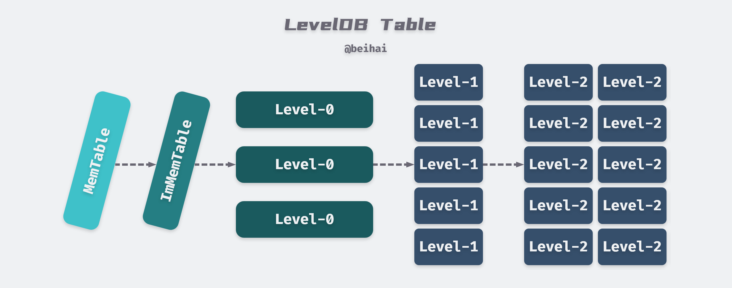
LevelDB can have 7 levels of SSTable at most, among which Level-0 is special, it is formed by dumping ImMemTable to disk directly, and each file size is about 4MB, while Level1 to Level6 are merged from the upper level, and each SSTable file size is 2MB, the total file size of Level1 is The total file size of Level1 is 10MB, then each level is 10 times larger than the previous one, and Level6 reaches 1TB.

Unlike the LSM-Tree paper description, LevelDB increases the number and total size of files in each level without increasing the SSTable file size.

Minor Compaction

When the MemTable is full and there are not many Level-0 files and there is no background merge thread to do the merge, it is frozen into ImMemTable and the function MaybeScheduleCompaction() is called to start a Detach thread to merge ImMemTable into SSTable. This process is called Minor Compaction. The effect of Detach is to separate the main thread from the child thread, both of which run at the same time, so that when the main thread ends, the process also ends, but the child thread continues to run in the background. This way, even if the main thread is aborted due to an error, it will not affect the merged thread in the background. When the child thread finishes running, the resources are reclaimed by the runtime library.

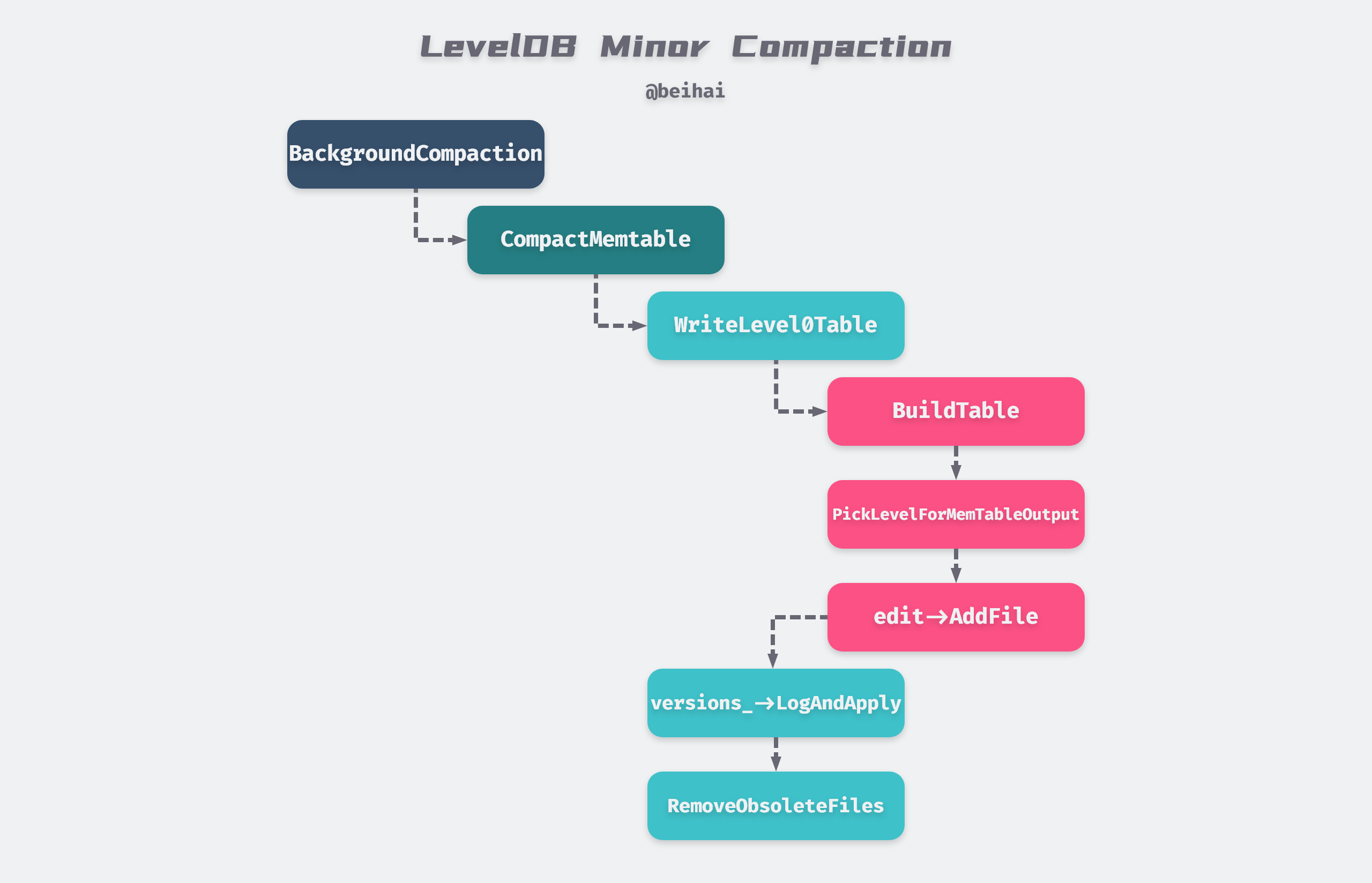
The background merge thread goes through a series of function calls and conditional judgments shown above, and will eventually enter DBImpl::WriteLevel0Table(), a function that first builds a new SSTable, maintains the file’s metadata, and updates the maximum and minimum key-value pairs for this file. When we look for data, comparing the bounding key-value pairs of this file will determine if it contains the data for the query.

 1
 2
 3
 4
 5
 6
 7
 8
 9
10
11
12

Status DBImpl::WriteLevel0Table(MemTable* mem, VersionEdit* edit, Version* base) {
  FileMetaData meta;
  meta.number = versions_->NewFileNumber();
  Iterator* iter = mem->NewIterator();
  BuildTable(dbname_, env_, options_, table_cache_, iter, &meta);

  const Slice min_user_key = meta.smallest.user_key();
  const Slice max_user_key = meta.largest.user_key();
  int level = base->PickLevelForMemTableOutput(min_user_key, max_user_key);
  edit->AddFile(level, meta.number, meta.file_size, meta.smallest, meta.largest);
  return Status::OK();
}

At the end of the process, the Version::PickLevelForMemTableOutput function is called to calculate which level the new SSTable file should be written to, and the judgment process is shown in the following figure.

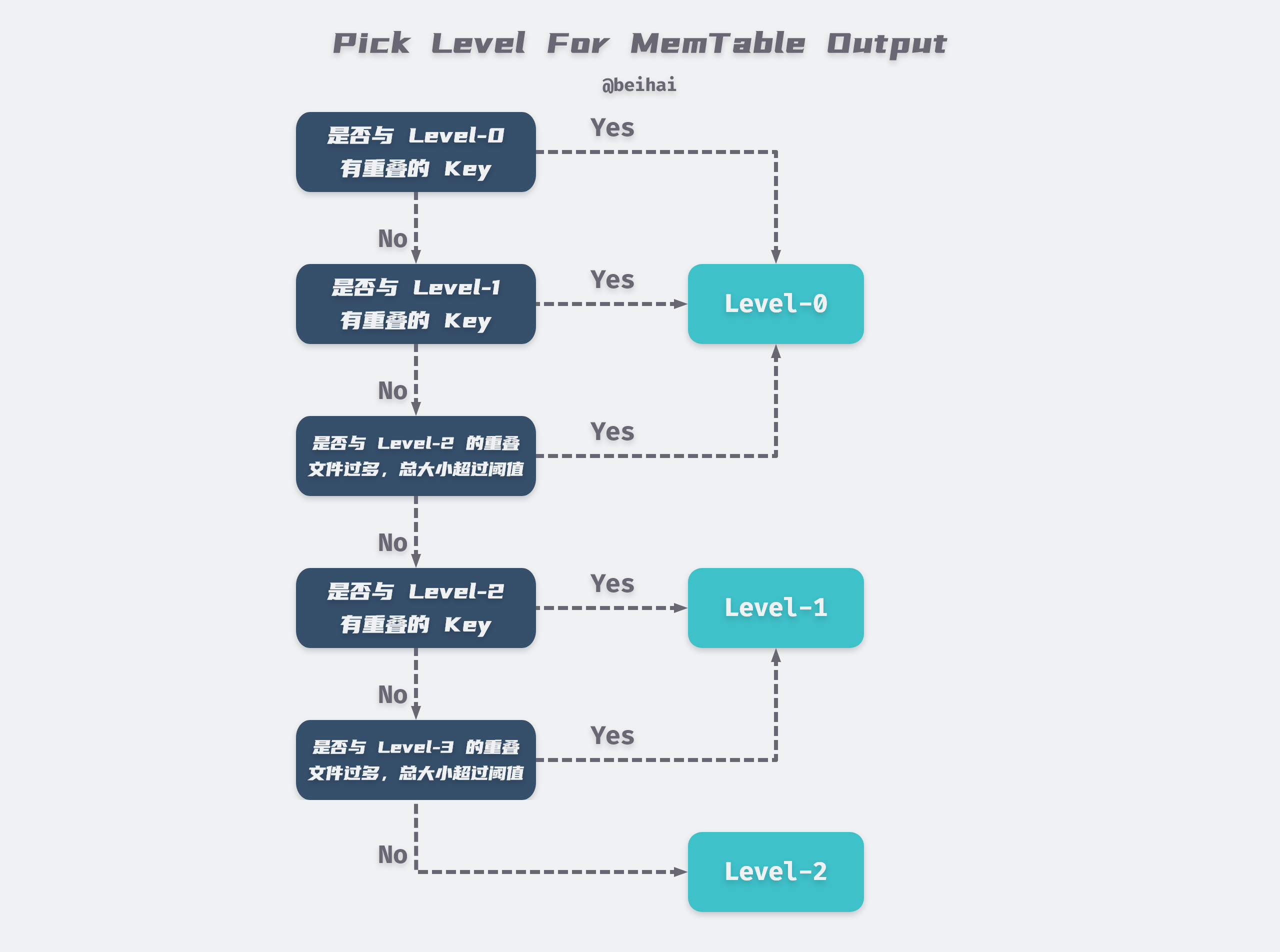
After the ImMemTable drop generates a new ldb file, the current version information is updated and some useless files are deleted, and the run ends here with a complete Minor Compaction. As you can see, in most cases ImMemTable will be dumped directly to Level-0, and may be merged to Level-1 and Level-2.

From the above figure, we can see that Level-0 does not consider the duplication of data between different files. So when we read the data, we always need to read all the files of Level-0, which is not friendly to read operation.

LevelDB mitigates this problem by setting a series of limits on the number of files in Level-0.

1. the number of Level-0 files exceeds 4, merged into Level-1.
2. more than 8 Level-0 files will delay writing key-value pairs by 1ms, slowing down the writing speed.
3. stop writing if the number of Level-0 files exceeds 12.

1
2
3
4
5
6
7
8

// Level-0 compaction is started when we hit this many files.
static const int kL0_CompactionTrigger = 4;

// Soft limit on number of level-0 files.  We slow down writes at this point.
static const int kL0_SlowdownWritesTrigger = 8;

// Maximum number of level-0 files.  We stop writes at this point.
static const int kL0_StopWritesTrigger = 12;

Major Compaction

When the number of files at a level exceeds a threshold, the SSTable files from that level are merged with the SSTable files from the higher level to become the new Level+1 files, a process called Major Compaction.

There are two types of trigger conditions for this process.

• The number of Level-0 files exceeds 4 or the total file size at a level exceeds a threshold.
• Too many invalid accesses (seek) to a file. Except for Level-0, SSTable files at any level are ordered among themselves. However, the keys of two files in Level(N) and Level(N+1) may intersect. Because of this intersection, when we look for a certain Key value, the Level(N) lookup is unsuccessful, so we have to look for it in Level(N+1), so this lookup causes more time consuming due to the overlapping range of keys in different levels. Therefore, LevelDB sets up an allowed_seeks for each SSTable after it is created for 100 times, and when allowed_seeks is < 0, it will trigger the merge with higher levels and merge the file to reduce the number of lookups for future queries.

Due to the specificity of Level-0, the Major Compaction process is also divided into two main types.

1. Level-0 and Level-1

   Select a Level-0 file, find a Level-1 file with duplicate Key, then find all Level-0 files with duplicate Key, and finally merge all Level-0 files and Level-1 files into a new Level-1 file.

2. Level-N and Level-(N+1)

   Select a Level-N file and find all the Level-(N+1) files with duplicate keys with that Level-N file to merge.

File Format

The format of an SSTable file is described in the LevelDB document table_format.md. Internally, an SSTable file consists of a series of 4KB-sized data blocks. The SSTable uses an index to locate the data blocks: when the SSTable file is opened, the index is loaded into memory and the location of the data blocks is then located according to the index. Each lookup can be done with a single disk search, first finding the location of the block in the index in memory using a dichotomous lookup, and then reading the corresponding block from the hard disk. We can also choose to cache the entire SSTable in memory so that we don’t have to access the hard disk.

The size of a data block is not a fixed length, but a threshold value, and a key-value pair is not stored across blocks. When the total length of all key-value pairs in a Block exceeds the threshold, LevelDB will create a new Block for storage.

For self-explanation of the file, the SSTable has an internal BlockHandle pointer to other locations in the file to indicate the start and end of a segment, and it has two member variables offset_ and size_ that record the start and length of a data block, respectively.

1
2
3
4
5

class BlockHandle {
private:
  uint64_t offset_;
  uint64_t size_;
};

The detailed format of the final SSTable file is shown above, with each section corresponding to the following meaning.

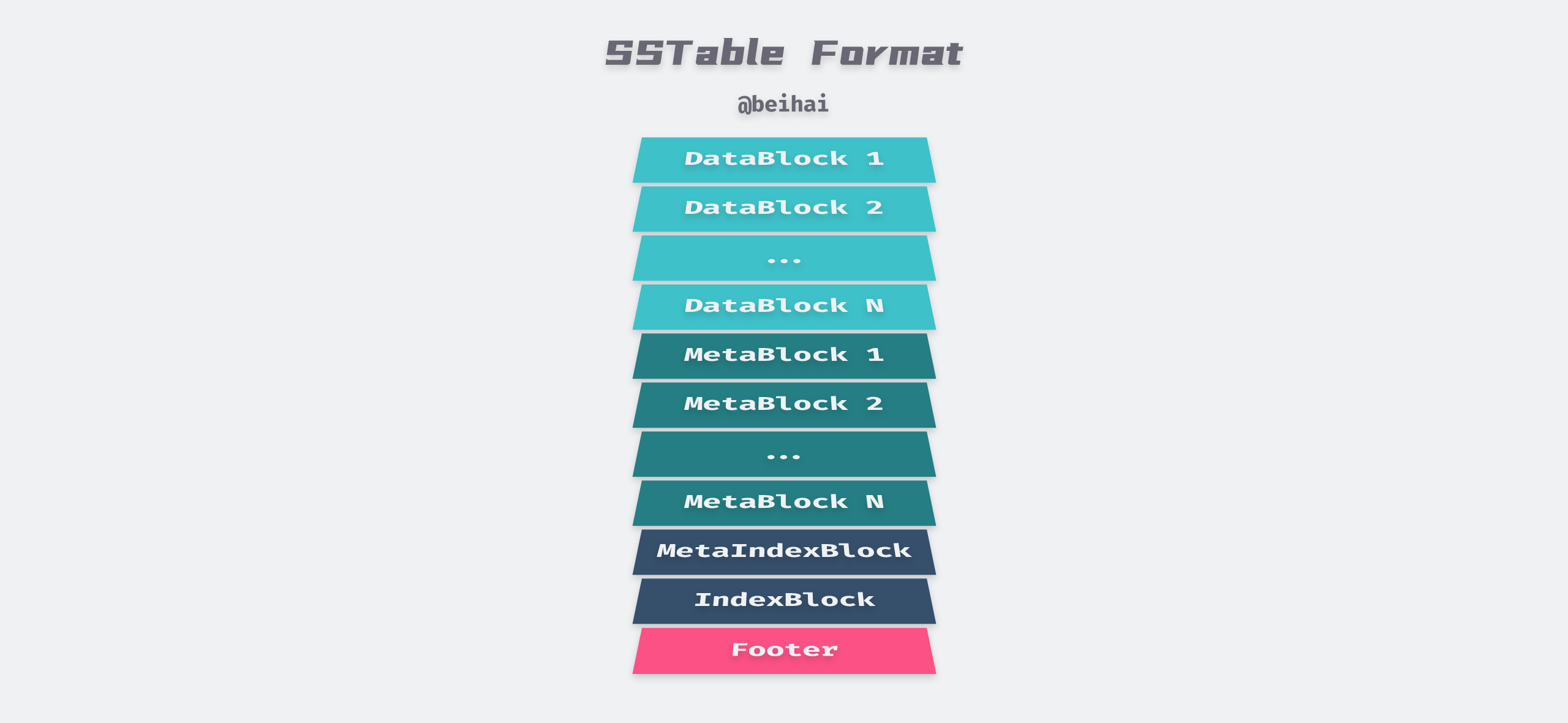
• The sequence of key-value pairs is stored in an ordered manner, divided into multiple data blocks, each of which is formatted and stored in a DataBlock.
• Each DataBlock corresponds to a MetaBlock, storing the Bloom Filter of the data block, and we can also customize our own filters for LevelDB.
• followed by a MetaIndexBlock, which is the entry point for other MetaBlocks, the stored Key is the name of this MetaBlock, and the value is a pointer BlockHandle to this MetaBlock.
• an index block IndexBlock, which contains the entry for each DataBlock, the Key is a string greater than or equal to the last key of the current DataBlock, before the first key of successive DataBlocks, and the value is a BlockHandle pointing to this DataBlock.
• At the end of the file is a filled-length Footer with a fixed length of 48 Bytes, containing the meta-index block and the BlockHandle of the index block, and a magic number.

A uint64 integer encoded with varint64 takes up to 10 bytes, and a BlockHandle contains two varint64 types, so a BlockHandle can take up to 20 bytes. So the maximum size of MetaIndex_Handle and Index_Handle is 40 bytes. 8 bytes for Magic Number, which is a fixed value to check if the file is an SSTable file when reading, and Padding is used to fill in the variable length integer part to 40 bytes.

The Footer of SSTable file can decode the BlockHandle of IndexBlock and MetaIndexBlock nearest to the Footer, so as to determine the position of these two components in the file, and then use these two index blocks to find out the position of other data blocks and filter blocks, so as to achieve the purpose of self-explanation of the file.

In addition, each SSTable file has its own max/min key pair. When we query the data, we can quickly determine whether we need to load the SSTable file into memory for searching by the max/min key pair, reducing I/O overhead.

Bloom Filter

A read operation must query the data of all SSTables at a given level. LevelDB reduces the number of hard disk accesses by allowing user programs to specify Bloom filters for SSTables of a particular locality group. We can use Bloom filters to determine whether an SSTable contains a particular key, significantly reducing the number of disk accesses for read operations at the cost of a small amount of memory capacity for storing Bloom filters. Using Bloom filters also implicitly achieves the goal of eliminating the need to access the hard disk most of the time when an application accesses a key-value pair that does not exist.

Bloom Filter is a probabilistic random data structure that acts similar to a hash table, it uses a bitmap to represent a set and can determine whether an element belongs to this set or not. The Bloom Filter has a certain misjudgment rate, when determining whether an element belongs to a set, it may mistake an element that does not belong to the set as belonging to the set, that is, it may have the following two situations.

1. the Bloom filter determines that a Key does not exist, then this Key must not exist in this set.
2. the Bloom filter determines that a key exists, then the key may exist.

The Bloom Filter is a bitmap structure with each bit being 0 at the beginning.

When the value X is inserted, X is hashed using k hash functions. The value obtained from the hash is then remapped with the capacity of the Bloom Filter, and the value of the bit represented by the remainder is set to 1.

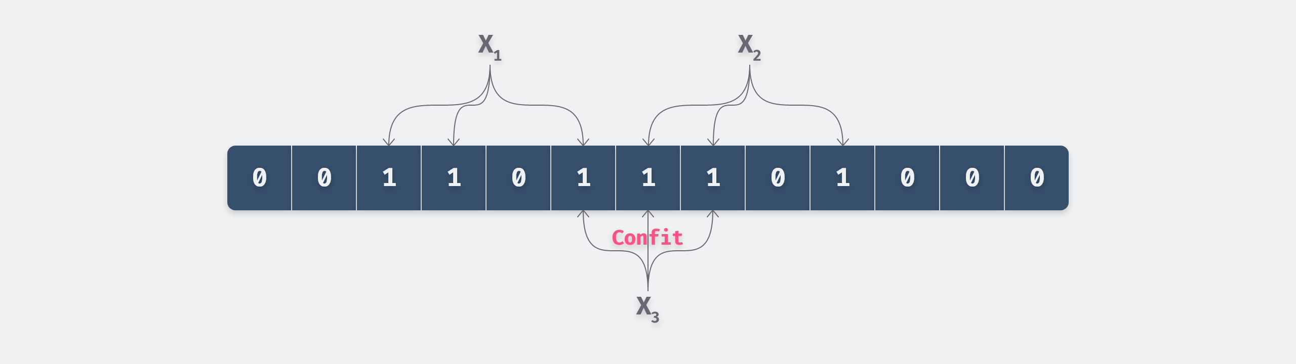
For example, in the above figure, we only inserted two values X1 and X2, although X3 is not inserted, but the query is Bloom filter will determine that it exists, which is the reason for the misjudgment.

The search process of Bloom filter is similar to the insertion process, which also uses k hash functions to hash the values that need to be found, and only if the value of each bit of the hash is 1, it means that the value may exist, and if the value of any bit is 0, it means that the value must not exist. For example, in the following figure, Y2 must not exist, while Y1 may exist.

LevelDB defines the filter base class FilterPolicy, according to which we can implement our own filters, or use the internal implementation of BloomFilterPolicy. The implementation of Bloom filter is relatively simple, and the main idea is to reduce the error rate.

If the bitmap has a total of m bits, the number of elements in the set is n, and the number of hash functions is k, then the larger m is, the larger k is, and the smaller n is, the smaller the false positive rate is. If m and n are deterministic, then the optimal number of hash functions k = ln2 × m/n. The file format of SSTable shows that Bloom Filter is not global, but generates its own filter for each data block, which avoids the increase of conflict rate due to the large n.

When we construct the new BloomFilterPolicy, the only parameter we need to pass is bits_per_key, which represents the ratio of the total length of the bitmap to the number of elements m/n, so that the optimal k value can be calculated.

1
2
3
4
5

  explicit BloomFilterPolicy(int bits_per_key) : bits_per_key_(bits_per_key) {
    k_ = static_cast<size_t>(bits_per_key * 0.69);  // 0.69 =~ ln(2)
    if (k_ < 1) k_ = 1;
    if (k_ > 30) k_ = 30;
  }

Knowing the above, it is easy to understand the CreateFilter() and KeyMayMatch() interfaces provided by BloomFilterPolicy, which represent the creation and query processes respectively. Note that a Bloom filter has a minimum bitmap of 64bits.

 1
 2
 3
 4
 5
 6
 7
 8
 9
10
11
12

void CreateFilter(const Slice* keys, int n, std::string* dst) const override {
size_t bits = n * bits_per_key_;

if (bits < 64) bits = 64;
size_t bytes = (bits + 7) / 8;
bits = bytes * 8;

for (int i = 0; i < n; i++) {
    uint32_t h = BloomHash(keys[i]);
    // write to dst
    }
}

TableCache

To improve the performance of read operations, LevelDB not only provides Bloom Filter to reduce the disk I/O of query process, but also uses cache to reside the frequently read SSTable in memory. Because of the localized nature of the program’s access to memory at runtime, the program will request a certain piece of memory very frequently, and if this piece of memory is cached after the first request, it will greatly improve the speed of data read afterwards. Therefore, whether the cache design is reasonable and effective lies in the high hit rate of the cache.

LevelDB provides TableCache class to cache SSTable files. You only need to provide the file_number and file_size of the file to return the corresponding Sorted Table object and its iterator. The TableCache is actually a layer of wrapper around the Cache class, similarly, the Cache class is an abstract class, and callers can either customize their own cache implementation by inheriting from the Cache class or directly use the internal implementation of LRUCache.

 1
 2
 3
 4
 5
 6
 7
 8
 9
10
11
12
13
14
15
16

class TableCache {
 public:
  Iterator* NewIterator(const ReadOptions& options, uint64_t file_number,
                        uint64_t file_size, Table** tableptr = nullptr);
  Status Get(const ReadOptions& options, uint64_t file_number,
             uint64_t file_size, const Slice& k, void* arg,
             void (*handle_result)(void*, const Slice&, const Slice&));

 private:
  Status FindTable(uint64_t file_number, uint64_t file_size, Cache::Handle**);

  Env* const env_;
  const std::string dbname_;
  const Options& options_;
  Cache* cache_;
};

LRUCahce uses the Least Recently Used (LRU) algorithm, if a piece of data has been used recently, the probability of it being used in the future is equally high . LRUCahce relies on the Doubly Circular Linked List and hash table implementation, where the node information for both the Linked List and the hash table is stored in the LRUHandle structure, and access is done with a mutual exclusion lock.

 1
 2
 3
 4
 5
 6
 7
 8
 9
10
11
12
13
14
15

class LRUCache {
 private:
  void LRU_Remove(LRUHandle* e);
  void LRU_Append(LRUHandle* list, LRUHandle* e);
    
  void Ref(LRUHandle* e);
  void Unref(LRUHandle* e);
  
  mutable port::Mutex mutex_;
  size_t usage_ GUARDED_BY(mutex_);

  LRUHandle lru_ GUARDED_BY(mutex_);
  LRUHandle in_use_ GUARDED_BY(mutex_);
  HandleTable table_ GUARDED_BY(mutex_);
};

The linked list in-use stores the data currently being referenced by the application, and another linked list lru caches the data in the order of access time, with each data being added or removed by the Ref() and Unref() functions, respectively, and completing the node switching between in-use and lru. When we need to use the LRU algorithm to eliminate data, we only need to eliminate the data on the lru linked list that is sorted next.

The hash table is used to quickly find out if a Key exists in the cache, and if it does, it returns a LRUHandle* pointer directly to the upper-level program. The hash table uses the classic array + linked list implementation with a load factor of 1. If the number of elements currently inserted exceeds the length of the array, it will be expanded, doubling the capacity each time.

1
2
3
4
5
6
7
8

Cache::Handle* LRUCache::Lookup(const Slice& key, uint32_t hash) {
  MutexLock l(&mutex_);
  LRUHandle* e = table_.Lookup(key, hash);
  if (e != nullptr) {
    Ref(e);
  }
  return reinterpret_cast<Cache::Handle*>(e);
}

To avoid storing too much data in one LRUCahce, LevelDB uses a sharded LRUCache ShardedLRUCache, which is also simple to implement, creating 16 LRUCahce objects at the same time, and then placing specific cached data into the corresponding LRUCahce objects via the Shard() function.

 1
 2
 3
 4
 5
 6
 7
 8
 9
10
11

static const int kNumShardBits = 4; // 用 4 个二进制位存储缓存片的数量，也就是 16 个缓存片
static const int kNumShards = 1 << kNumShardBits;

class ShardedLRUCache : public Cache {
 private:
  LRUCache shard_[kNumShards];
  port::Mutex id_mutex_;
  uint64_t last_id_;

  static uint32_t Shard(uint32_t hash) { return hash >> (32 - kNumShardBits); }
};

Summary

LSM-Tree and B-Tree and their variants are widely used in storage systems. Unlike the high read performance of B-Tree, LSM-Tree greatly improves the write ability of data, but at the expense of partial read performance, so this structure is usually suitable for scenarios with more writes and fewer reads.

I have read and analyzed the source code of LevelDB to get a better understanding of the design of this data structure. This article covers MemTable, SSTable, pre-written log, etc., and analyzes Bloom Filter and TableCache used by LevelDB to improve readability, but does not introduce version control and data recovery related content.

LevelDB is written by Jeff Dean, the author of BigTable, and the code is very elegant and makes a lot of use of PImpl and OOP concepts. It is a very good project to learn C++ programming. There are more articles about LevelDB source code analysis on the web, you can Google to learn what is not covered or not clearly described in the article.

References

• https://wingsxdu.com/posts/database/leveldb/#major-compaction
• The Log-Structured Merge-Tree (LSM-Tree)
• Bigtable: A Distributed Storage System for Structured Data
• Log Structured Merge Trees
• LevelDB Source Code Analysis
• SSTable in LevelDB
• leveldb source code reading (IV) - table cache implementation