Pandas Data Processing Concise Tutorial

When using Python to process and analyze data, the most used is Pandas. Since Pandas is a very powerful tool and involves a lot of functions, it is often necessary to consult the documentation when using it. Here is a record of some of the functions and knowledge points that you commonly use.

Introduction to Pandas

Pandas is a data analysis package for python, originally developed by AQR Capital Management in April 2008 and open sourced out at the end of 2009, and is now continued to be developed and maintained by the PyData development team, which focuses on Python data package development and is part of the PyData project. pandas was originally was originally developed as a financial data analysis tool, so pandas provides good support for time series analysis.

Pandas is suitable for working with the following types of data.

• Tabular data with heterogeneous columns, similar to SQL or Excel tables
• Ordered and unordered (non-fixed frequency) time series data
• Matrix data with row labels, including isomorphic or heterogeneous data
• Any other form of observations, statistical data sets, which do not need to be pre-tagged when transferred to the Pandas data structure.

Advantages of Pandas.

• Handles missing data in floating-point and non-floating-point data, represented as NaN
• Variable size: insert or delete columns of multidimensional objects such as DataFrame
• Automatic, explicit data alignment: explicitly align objects to a set of labels, or ignore labels and automatically align to data in Series, DataFrame calculations
• Powerful, flexible group by functionality: split-apply-combine datasets, aggregate, transform data
• Easily convert irregular, differently indexed data from Python and NumPy data structures into DataFrame objects.
• Slicing, fancy indexing, and subset decomposition of large datasets based on smart tags
• Intuitively merge and join datasets
• Flexible reshape and pivot datasets
• Axis support for structured labels: multiple labels for one scale
• Mature IO tools: read data from text files (CSV and other files with delimiter support), Excel files, databases, and other sources, and save/load data using the ultra-fast HDF5 format
• Time series: Support date range generation, frequency conversion, moving window statistics, moving window linear regression, date displacement, and other time series functions.

Series And DataFrame

Pandas is based on NumPy and integrates well with other third-party scientific computing support libraries.

• A Series is a one-dimensional array-like object that consists of a set of data and a set of data sticky notes (i.e., an index) associated with it, producing the simplest Series from a set of data alone.
• A DataFrame is a tabular data containing an ordered set of columns, each of which can be a different type of value. a DataFrame can be thought of as a dictionary of multiple Series that share a common index.

Series is a one-dimensional structure, each column of DataFrame is a series (Series), the series structure only has row index (row index), no column name (column name), but the series has Name, dtype and index attributes, where the Name attribute refers to the name of the series. dtype attribute is the type of the sequence value, and index attribute is the index of the sequence. The data type of the data stored in the sequence is the same.

DataFrame stores two-dimensional data. The structure of DataFrame consists of row and column, each row has a row label, each column has a column label, and the row and column are called axis, and the row label and column label are called axis label. Normally, column label is a text type, which is the column name, and row label is a numeric type, which is also called row index.

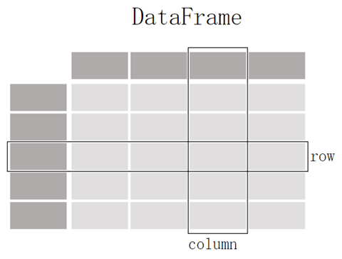
For these two data structures, there are two most basic concepts: Axis and Label. For two-dimensional data structures, Axis refers to the rows and columns, and Axis Label refers to the row index and column name, and the data structure to store Axis Label is Index structure. Each row has an index by which the row can be located; each column has a column name by which the column can be located; and the data value of a unique data point (cell) can be uniquely located by the row index and column name.

Axis Labels

The data structure for storing axis labels is Index. For data frames, the row labels (i.e., row indexes) and column names (i.e., column indexes) are stored by Index objects; for sequences, the row indexes are stored by Index objects. The Index object is unmodifiable, similar to a fixed-size array.

For indexes, they can also be accessed by the ordinal number, which is automatically generated and starts from 0.

The most important roles of axis labels are.

• Uniquely identifies the data and is used to locate it
• For data alignment
• Get and set a subset of the data set.

Both data frame and sequence objects have an attribute index for getting row labels and, for data frames, a columns attribute for getting column labels:.

1
2
3
4
5

>>> df.index
RangeIndex(start=0, stop=3, step=1)

>>>df.columns
Index(['Name', 'Age', 'Sex'], dtype='object')

Pandas library axis=0, axis=1 axis usage

When I first learned Pandas, I was confused by axis=0 or axis=‘index’, axis=1 or axis=‘columns’, and I often even thought that the book was written wrong and a bit counter-intuitive.

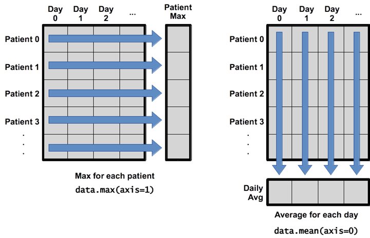
In the figure above.

• axis = 1: means finding the maximum of all columns along the rows, which represents the horizontal axis.
• axis = 0: is the average of all rows along the columns, representing the vertical axis.

Pandas row, column, and index operations

Pandas Row, Column, Index Routines

1
2
3
4
5
6
7
8
9

print(df.columns)  # 输出列名
df.columns = ['a', 'b', 'c']  # 重命名列名
df = df[['a', 'b', 'c']]  # 只选取想要的列

df = df.transpose()  # 行列转换
df = df.T  # 行列转换的简写方式

df = df.set_index('c')  # 以c列作为索引
df.reset_index() # 重新变为默认的数值索引

loc and iloc in Pandas

The difference between loc and iloc.

• .loc is mainly based on labels (label), including row labels (index) and column labels (columns), i.e., row names and column names, which can be used loc[index_name,col_name]
• .iloc is a position-based index, using the index number of the element on each axis for selection

Example code.

 1
 2
 3
 4
 5
 6
 7
 8
 9
10
11
12
13
14

# .loc的用法
df.loc[3]  # 选择index为3的一行，这里的’3’是index的名称，而不是序号
df.loc['a']  # 获取index是a的某一行
df.loc[['a', 'b', 'c']]  # 获取index为a,b,c的行
df.loc['c':'h']  # 获取c到h行，包含c和h（左闭右闭）
df.loc[df['A'] > 5]  # 筛选出所有A列>5的行
df.loc[df['A'] > 5, ['C', 'D']]  # 筛选出所有A列>5的行的C和D列

# .iloc的用法
df.iloc[3] # 选择第四行，下标从0开始
df.iloc[[1,3,5]] # 选择第2、4、6行
df.iloc[0:3] # 选择1~3行，和loc不同的是这里是左闭右开
df.iloc[0:3,1:3] # 选择1~3行,2~3列
df.iloc[df['A'] > 5]  # 同上

Commonly used operations.

1
2

X = df.iloc[:, :-1]
y = df.iloc[:, -1]

Pandas and Time Series

Relying on NumPy’s datetime64, timedelta64, and other data types, pandas can handle all kinds of time series data, and can also call the time series functions of Python support libraries such as scikits.timeseries.

 1
 2
 3
 4
 5
 6
 7
 8
 9
10
11
12
13
14
15
16
17
18
19
20
21
22

# 解析时间格式字符串、np.datetime64、datetime.datetime 等多种时间序列数据。
dti = pd.to_datetime(['1/1/2018', np.datetime64('2018-01-01'), datetime.datetime(2018, 1, 1)])

# 生成 DatetimeIndex、TimedeltaIndex、PeriodIndex 等定频日期与时间段序列。
dti = pd.date_range('2018-01-01', periods=3, freq='H')

# 处理、转换带时区的日期时间数据。
dti = dti.tz_localize('UTC')
dti.tz_convert('US/Pacific')

# 按指定频率重采样，并转换为时间序列。
idx = pd.date_range('2018-01-01', periods=5, freq='H')
ts = pd.Series(range(len(idx)), index=idx)
ts.resample('2H').mean()

# 用绝对或相对时间差计算日期与时间。
friday = pd.Timestamp('2018-01-05')
print(friday.day_name())
saturday = friday + pd.Timedelta('1 day')
print(saturday.day_name())
monday = friday + pd.offsets.BDay() # 添加 1 个工作日，从星期五跳到星期一
print(monday.day_name())

Slicing for time-indexed data.

1
2
3
4
5
6

ts['2021'] # 查询整个2021年的
ts['2021-6'] # 查询 2021年6月的
ts['2021-6':'2021-10'] # 6月到10月的
dft['2013-1':'2013-2-28 00:00:00'] # 精确时间
dft['2013-1-15':'2013-1-15 12:30:00']
dft.loc['2013-01-05']

Pandas data types

The main data types in Pandas are.

• float
• int
• bool
• datetime64[ns]
• datetime64[ns, tz]
• timedelta64[ns]
• timedelta[ns]
• category
• object

The default data types are int64 and float64, and the literal type is object.

Correspondence with Python and NumPy types.

Commonly used methods.

1
2
3

df.dtypes  # 各字段的数据类型
df['a'].dtype  # 某个字段的类型
df['a'].astype(float)  # 转换类型

Pandas data acquisition and processing

In daily work, the most used is to read data from Excel and CSV files using Pandas. Another common operation is the conversion into a DataFrame by means of a dict list.

1
2
3
4
5
6
7
8

import pandas as pd

d = [{'points': 50, 'time': '5:00', 'year': 2010},
     {'points': 25, 'time': '6:00', 'month': "february"},
     {'points': 90, 'time': '9:00', 'month': 'january'},
     {'points_h1': 20, 'month': 'june'}]

df = pd.DataFrame(d)

In addition to this, there are the usual operations such as merging and joining DataFrames in Pandas and reading database data in Pandas.

Pandas for exploring data

View Data Basics

View, check data.

• head(n): view the first n rows of the DataFrame object
• tail(n): view the last n rows of the DataFrame object
• shape(): view the number of rows and columns
• info(): view index, data type and memory information
• describe(): view the summary statistics of numeric columns
  • describe(include=[np.number]) # Specify the number type
  • describe(include=[np.object]) # Specify the object type
  • describe(include=[‘category’]) # Specify the column name
• value_counts(dropna=False): view the unique values and counts of the Series object
• apply(pd.Series.value_counts): view the unique values and counts of each column in the DataFrame object
• unique: return the unique value
• corr(): return the column-to-column correlation

1

DataFrame.corr(method='pearson', min_periods=1)

Parameter description.

• method: optional values are {‘pearson’, ‘kendall’, ‘spearman’}
• min_periods: the minimum amount of data to sample

Handling of abnormal data

Checking for null values

There are two methods for checking null values in Pandas, pandas.DataFrame.isna() and pandas.DataFrame.isnull(), both of which I use exactly the same way.

Example usage.

• isna().sum()

Value substitution

Example.

• replace(’-’,’np.nan’): replace ‘-’ with a Null value
• replace(1,‘one’): replace all values equal to 1 with ‘one’
• replace([1,3],[‘one’,’three’]): replace 1 with ‘one’ and 3 with ’three’

Delete null values

1

DataFrame.dropna(axis=0, how='any', thresh=None, subset=None, inplace=False)

Parameter description.

• axis: it determines whether the axis is a row or a column.
  • If it is 0 or ‘index’, then it will delete the row containing the missing value.
  • If it is 1 or ‘column’, then it will delete the column containing the missing value. By default, its value is 0
• how: This parameter determines how the function deletes rows or columns. It accepts only two strings, either all or all. by default, it is set to any.
  • any - if there is any null value in the row or column, it will be deleted.
  • all - if all values are missing from the row or column, it drops the row or column
• thresh: it is an integer that specifies the minimum number of non-missing values that prevent a row or column from being missing
• subset: it is an array with the names of the rows or columns, which specifies the deletion procedure
• inplace: it is a Boolean value that, if set to True, will change the caller DataFrame in place. by default, its value is False

Example.

• dropna(): delete all rows that contain null values
• dropna(axis=1): delete all columns that contain null values
• dropna(axis=1,fresh=n): delete all rows with less than n non-null values

Fill with empty values

1

DataFrame.fillna(value=None, method=None, axis=None, inplace=False, limit=None, downcast=None)

Parameter Description.

• value: the value used to fill the null value
• method: {‘backfill’, ‘bfill’, ‘pad’, ‘ffill ‘, None}, default None, pad/ffill means backfill, backfill/bfill means forward fill
• axis: the axis along which the missing value is filled
• inplace: boolean, default is False. if True, fill in place.
• limit: int, default is None, if method is specified, then this is the maximum number of consecutive NaN values to be filled forward/backward
• downcast: dict, default None, the item in the dictionary is a type-down conversion rule.

Example.

• fillna(x): replace all null values in the DataFrame object with x
• fillna(s.mean()): fill with the mean value
• fillna(s.median()): fill with the median

Remove duplicates

1

DataFrame.drop_duplicates(subset=None, keep='first', inplace=False, ignore_index=False)

Parameter Description.

• subset: Enter the name of the column to be de-duplicated, default is None
• keep: There are three optional parameters: ‘first’, ’last’, False, and the default value is ‘first’. Among them, the
  • first means: Keep the first occurrence of duplicate rows, and delete the following duplicate rows.
  • last means: Remove duplicates and keep the last occurrence.
  • False means: Remove all duplicates.
• inplace: Boolean value, default is False, whether to remove duplicate items directly on the original data or return a copy after removing duplicate items.

Example.

1

df.drop_duplicates(subset=['A','B'],keep='first',inplace=True)

Summary statistics of data

Commonly used statistical functions in Pandas.

• .count() # Non-null element count
• .size() # count with NaN
• .min() # min value
• .max() # maximum value
• .idxmin() # the position of the minimum value, similar to the min function in R
• .idxmax() # location of the maximum value, similar to the max function in R
• .quantile(0.1) # 10% quantile
• .sum() # summation
• .mean() # mean value
• .median() # median
• .mode() # plurality
• .var() # variance
• .std() # standard deviation
• .mad() # mean absolute deviation
• .skew() # skewness
• .kurt() # kurtosis

When we want to view the data in each column of the DataFrame, we can customize a function to conveniently summarize the statistical indicators together (the effect is similar to df.describe()).

 1
 2
 3
 4
 5
 6
 7
 8
 9
10
11
12
13
14
15

import pandas as pd
import numpy as np


def status(x):
    return pd.Series(
        [x.count(), x.min(), x.idxmin(), x.quantile(.25), x.median(), x.quantile(.75), x.mean(), x.max(), x.idxmax(),
         x.mad(), x.var(), x.std(), x.skew(), x.kurt()],
        index=['总数', '最小值', '最小值位置', '25%分位数', '中位数', '75%分位数', '均值', '最大值', '最大值位数', '平均绝对偏差', '方差', '标准差', '偏度',
               '峰度'])

if __name__ == "__main__": 
    # df = pd.DataFrame(status(d1))
    df = pd.DataFrame(np.array([d1, d2, d3]).T, columns=['x1', 'x2', 'x3'])
    df.apply(status)

Groupby() in Pandas

In the simplest way, specify the columns and statistical functions to be grouped.

1

df.groupby(by=['col1','col2']).size()

Usually the values counted do not have column names, which can be specified by this method.

1

df.groupby(by=['col1', 'col2']).size().reset_index(name='counts')

groupby combined with agg for aggregation.

1

df[['col1', 'col2', 'col3', 'col4']].groupby(['col1', 'col2']).agg(['mean', 'count'])

The above code is similar to the following SQL.

1

SELECT col1, col2, avg(col1), count(col2) FROM df GROUP BY col1, col2

Add column name.

1

key1 = df.groupby(["key1"], as_index=False)["data1"].agg({"col_name": "count"})

Sorting sort_values() in Pandas

Usage.

• sort_values(col1): sort data by column col1, ascending by default
• sort_values(col2, ascending=False): sort data by column col1 in descending order
• sort_values([col1,col2], ascending=[True,False]): sort the data by column col1 ascending first, then by column col2 descending

Pandas Dataframe traversal

1
2

for index, row in df.iterrows():
    print(row['c1'], row['c2'])

Pandas’ apply function

The apply() method of Pandas is used to call a function (Python method) that allows this function to perform batch processing on data objects.

1

DataFrame.apply(func, axis=0, raw=False, result_type=None, args=(), **kwargs)

Parameter Description.

• func: function to be applied to each column or row.
• axis: {0 or ‘index’, 1 or ‘columns’}, default is 0
  • 0 or ‘index’: function to be applied to each column.
  • 1 or ‘columns’: apply the function to each row.
• raw: Determines if rows or columns are passed as Series or ndarray objects.
  • False: Passes each row or column as a Series to the function.
  • True: The passed function will instead receive an ndarray object. You will get better performance if you only apply the NumPy reduction function.
• result_type: {’expand’, ‘reduce’, ‘broadcast’, None}, these only work if axis=1 (column).
  • ’expand’: list-like results will become columns.
  • ‘reduce’: If possible, a sequence is returned instead of the expanded list-like result. This is the opposite of ’expand’.
  • ‘broadcast’: the result will be broadcast to the DataFrame’s original

Example.

 1
 2
 3
 4
 5
 6
 7
 8
 9
10
11
12
13
14

ser.apply(fun) # 自定义
ser.apply(max) # python 内置函数
ser.apply(lambda x: x*2) # lambda
ser.apply(np.mean) # numpy 等其他库的函数 ufunc
ser.apply(pd.Series.first_valid_index) # Pandas 自己的函数
ser.apply('count') # Pandas 自己的函数
ser.apply('shape') # Pandas 自己的属性
ser.apply('tan') # numpy 的 ufunc 名
# 多个函数
ser.apply([sum, 'count']) # 相当于 .aggregate, 即.agg
ser.apply(np.array(["sum", "mean"]))
ser.apply({'Q1':sum, 'Q2':'count'}) # 同上
#SQL中row_number()的实现
df['Rank'] = df.groupby(by=['交易日期'])['交易时间'].apply(lambda x: x.rank(ascending=False))

Pandas panning functions shift() and diff()

The shift() function

shift () function is the main function is to make the data in the data box to move, if freq = None, according to the axis setting, line index data remain unchanged, column index data can be moved up and down on the line or left and right on the column; if the line index for the time series, you can set the freq parameter, according to the periods and freq parameter value combination, so that each time the line index occurs periods * freq offset scroll, column index data will not move.

1

DataFrame.shift(periods=1, freq=None, axis=0, fill_value=<no_default>)

Parameter Description.

• period: the magnitude of the move, can be positive or negative, the default value is 1,1 means move once, note that here the move is all data, and the index is not moved, after the move there is no corresponding value, the value is assigned to NaN.
• freq: DateOffset, timedelta, or time rule string, optional parameter, default value is None, only for time series, if this parameter exists, then the time index will be moved according to the parameter value, and the data value is not changed.
• axis: {0, 1, ‘index’, ‘columns’}, indicates the direction of moving, if it is 0 or ‘index’ means move up and down, if it is 1 or ‘columns’, it will move left and right.
• fill_value: the value to be filled for empty rows

diff() function

From the official description has been very clear to know the relationship of its shift function: df.diff () = df - df.shift ()

1

DataFrame.diff(periods=1, axis=0)

Parameter description.

• periods: the magnitude of the move, int type, default value is 1.
• axis: the direction to move, {0 or ‘index’, 1 or ‘columns’}, if it is 0 or ‘index’, then move up and down. If it is 1 or ‘columns’, then move left and right.

Reference links.

• Pandas API reference