Basemap Introduction

Basemap is a toolkit under the Python visualization library Matplotlib. its main function is to draw 2D maps, which are important for visualizing spatial data. basemap itself does not do any plotting, but provides the ability to transform coordinates into one of 25 different map projections. Matplotlib can also be used to plot contours, images, vectors, lines, or points in transformed coordinates. basemap includes the GSSH coastline dataset, as well as datasets from GMT for rivers, states, and national boundaries. These datasets can be used to plot coastlines, rivers, and political boundaries on a map at several different resolutions. basemap uses the Geometry Engine-Open Source (GEOS) library at the bottom to clip coastline and boundary features to the desired map projection area. In addition, basemap provides the ability to read shapefiles.

Installing Basemap

Basemap cannot be installed using pip install basemap. If Anaconda is installed, you can install basemap using canda install basemap.

For cases where it cannot be installed, you can download the compiled installation package: https://www.lfd.uci.edu/~gohlke/pythonlibs/. You need to install pyproj before installing basemap.

After installation, the following error will be reported when executing the code: KeyError: ‘PROJ_LIB’

Solution.

1
2
3
import os
os.environ["PROJ_LIB"] = r"D:\ProgramData\Anaconda3\pkgs\proj4-5.2.0-h6538335_1006\Library\share"; #fixr
from mpl_toolkits.basemap import Basemap

Or set it directly in the environment variable.

Use of Basemap

Some example objects in basemap.

  • contour() : draw contour lines.
  • contourf() : draw filled contours.
  • imshow() : draw an image.
  • pcolor() : draw a pseudocolor plot.
  • pcolormesh() : draw a pseudocolor plot (faster version for regular meshes).
  • plot() : draw lines and/or markers.
  • scatter() : draw points with markers.
  • quiver() : draw vectors.(draw vector map, 3D is surface map)
  • barbs() : draw wind barbs (draw wind plume map)
  • drawgreatcircle() : draw a great circle (draws a great circle route)

Basemap Basic Usage

1
2
3
4
5
6
7
8
9
import warnings
warnings.filterwarnings('ignore') 
from mpl_toolkits.basemap import Basemap
import matplotlib.pyplot as plt

map = Basemap()
map.drawcoastlines()
# plt.show()
plt.savefig('test.png')

Code description.

  • The first line of code introduces the Basemap library and matplotlib, both of which are required.
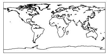
  • This map is created by the Basemap class, which contains many properties. If you use the defaults, the map has lat=0 and lon=0 centers and displays the map using the normal cylindrical projection mode (Plate Carrée projection). The projection formula is as simple as it can be: x=lon, y=lat. However, this projection is neither equal angle nor equal product, especially at high latitudes, and it is not practical because it differs greatly from reality. Changing the projection of the map is very simple, just add the projection parameter and the lat_0, lon_0 parameters to Basemap().
  • In this example, the coastlines are drawn with the drawcoastlines() method, and the coastline data is already included in the library file by default.
  • Finally, use the methods in pyplot to display and save the image.

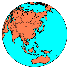
Changing the projection is easy, just let’s switch to another projection ortho below and see the effect. In addition we use the methods fillcontinents() and drawmapboundary() to fill in the colors of the ocean and earth.

1
2
3
4
5
6
map = Basemap(projection='ortho',lat_0=30, lon_0=120)
map.drawmapboundary(fill_color='aqua')
map.fillcontinents(color= 'coral',lake_color='aqua')
map.drawcoastlines()
map.drawcountries()
plt.show()

Projection types supported by Basemap.

1
2
import mpl_toolkits.basemap
print(mpl_toolkits.basemap.supported_projections)
 1
 2
 3
 4
 5
 6
 7
 8
 9
10
11
12
13
14
15
16
17
18
19
20
21
22
23
24
25
26
27
28
29
30
31
32
33
34
cyl              Cylindrical Equidistant                 
merc             Mercator                                
tmerc            Transverse Mercator                     
omerc            Oblique Mercator                        
mill             Miller Cylindrical                      
gall             Gall Stereographic Cylindrical          
cea              Cylindrical Equal Area                  
lcc              Lambert Conformal                       
laea             Lambert Azimuthal Equal Area            
nplaea           North-Polar Lambert Azimuthal           
splaea           South-Polar Lambert Azimuthal           
eqdc             Equidistant Conic                       
aeqd             Azimuthal Equidistant                   
npaeqd           North-Polar Azimuthal Equidistant       
spaeqd           South-Polar Azimuthal Equidistant       
aea              Albers Equal Area                       
stere            Stereographic                           
npstere          North-Polar Stereographic               
spstere          South-Polar Stereographic               
cass             Cassini-Soldner                         
poly             Polyconic                               
ortho            Orthographic                            
geos             Geostationary                           
nsper            Near-Sided Perspective                  
sinu             Sinusoidal                              
moll             Mollweide                               
hammer           Hammer                                  
robin            Robinson                                
kav7             Kavrayskiy VII                          
eck4             Eckert IV                               
vandg            van der Grinten                         
mbtfpq           McBryde-Thomas Flat-Polar Quartic       
gnom             Gnomonic                                
rotpole          Rotated Pole

How exactly to use and style can be tested for yourself.

Slightly more complex maps.

 1
 2
 3
 4
 5
 6
 7
 8
 9
10
11
12
13
14
15
import warnings
warnings.filterwarnings('ignore') 
from mpl_toolkits.basemap import Basemap
import matplotlib.pyplot as plt
import numpy as np

my_map = Basemap(resolution='i', projection='merc', llcrnrlat=10.0, urcrnrlat=55.0, llcrnrlon=60., urcrnrlon=140.0)
my_map.drawcoastlines()
my_map.drawcountries()
my_map.drawmapboundary()
my_map.fillcontinents(color='coral', lake_color='aqua')
my_map.drawmeridians(np.arange(0, 360, 30),labels=[True,True,True,True])
my_map.drawparallels(np.arange(-90, 90, 30),labels=[True,True,True,True])
my_map.drawmapboundary(color='k', linewidth=1.0, fill_color='b', zorder=None, ax=None)
plt.show()
  • The resolution parameter of the basemap class sets the resolution level, they are ‘c’ (original), ’l’ (low), ‘i’ (medium) ‘h’ (high), ‘f’ (full) or None (if no boundaries are used). This option is important, setting high resolution borders on the global map can be very slow.
  • We can zoom from to a specific area, here the parameters are.
    • llcrnrlat - latitude of the lower left corner
    • llcrnrlon - longitude in the lower left corner
    • urcrnrlat - latitude in the upper right corner
    • urcrnrlon - the longitude of the upper right corner
  • Longitude and latitude lines can be drawn with drawmeridians() and drawparallels().

Adding points and lines.

 1
 2
 3
 4
 5
 6
 7
 8
 9
10
11
12
13
14
15
16
17
18
from mpl_toolkits.basemap import Basemap
import matplotlib.pyplot as plt
import numpy as np

fig = plt.figure()
mymap = Basemap(llcrnrlon=-100.,llcrnrlat=20.,urcrnrlon=20.,urcrnrlat=60.,lat_0=40.,lon_0=-20.,lat_ts=20.)
# nylat, nylon are lat/lon of New York
nylat = 40.78; nylon = -73.98
# lonlat, lonlon are lat/lon of London.
lonlat = 51.53; lonlon = 0.08
mymap.scatter([nylon,lonlon],[nylat,lonlat], linewidths = 10, marker = 'o', color = 'red',s=20, zorder=40)
mymap.drawgreatcircle(nylon,nylat,lonlon,lonlat,linewidth=2,color='b')
mymap.plot([nylon,lonlon],[nylat,lonlat],linewidth=2,color='green',latlon='True')
mymap.drawcoastlines()
mymap.fillcontinents()
mymap.drawparallels(np.arange(10,90,20),labels=[1,1,0,1])
mymap.drawmeridians(np.arange(-180,180,30),labels=[1,1,0,1])
plt.show()

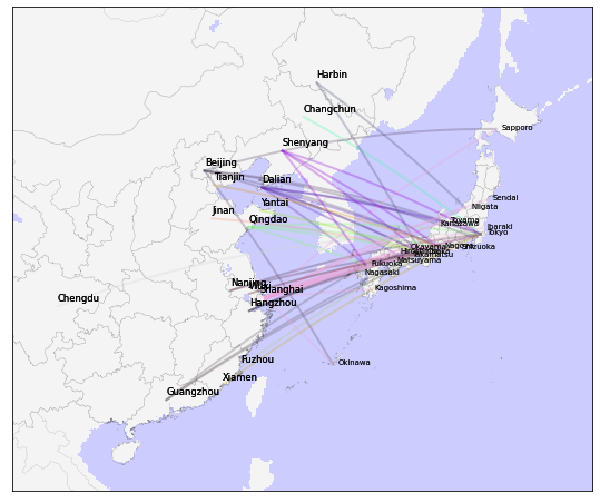
Basemap hands-on: Open Flights data visualization

The official website of Open Flights provides standalone text in the form of airports.dat, airlines.dat, routes.dat, here we use Data Quest provides a packaged .db file.

 1
 2
 3
 4
 5
 6
 7
 8
 9
10
11
12
13
14
15
16
17
18
19
20
21
22
23
24
25
26
27
28
29
30
31
32
33
34
35
36
37
38
39
40
41
42
43
44
45
46
47
48
49
50
51
52
53
54
55
56
57
58
59
60
61
62
63
64
65
66
67
68
69
70
71
72
73
74
75
76
77
78
79
80
81
82
83
84
85
86
87
88
89
import sqlite3
import pandas as pd
import numpy as np
from mpl_toolkits.basemap import Basemap
import matplotlib.pyplot as plt
import warnings
warnings.filterwarnings('ignore')

db = sqlite3.connect('flights.db')

# 获取所有中国机场数据
airports = pd.read_sql_query(
    """
    SELECT DISTINCT cast(latitude AS float) AS lat,
       cast(longitude AS float) lon
    FROM airports
    WHERE country = 'China';
    """,
    db
)

# 获取所有中日航线数据
routes = pd.read_sql_query(
    """
    SELECT DISTINCT cast(sa.latitude AS float) AS src_lat,
       cast(sa.longitude AS float) AS src_lon,
       cast(da.latitude AS float) AS dest_lat,
       cast(da.longitude AS float) AS dest_lon,
       sa.city as src_city,
       da.city as dest_city
    FROM routes
    INNER JOIN airports sa ON sa.id = routes.source_id
    AND sa.country = 'China'
    INNER JOIN airports da ON da.id = routes.dest_id
    AND da.country = 'Japan';
    """,
    db
)

# 加载行政区边界
chn = map.readshapefile('gadm36_CHN_shp/gadm36_CHN_1', 'chn', color='#555555', linewidth=0.1, ax=ax)
jpn = map.readshapefile('gadm36_JPN_shp/gadm36_JPN_1', 'jpn', color='#555555', linewidth=0.1, ax=ax)

# 将国内机场添加到地图
x, y = map(list(airports['lon']),list(airports['lat']))
map.scatter(x, y, 50, marker='.', color='b', alpha=0.1, ax=ax)


# 绘制中日航线
grouped = routes.groupby('src_city')
src_city_list = grouped.groups.keys()

colors_length = np.random.random((len(src_city_list), 3))
colors = dict([(city, color) for city, color in zip(src_city_list, colors_length)])

for key, group in grouped:
    for index, row in group.iterrows():
        map.drawgreatcircle(
            row['src_lon'],
            row['src_lat'],
            row['dest_lon'],
            row['dest_lat'],
            linewidth=2,
            c=colors[key],
            alpha=0.3,
            ax=ax
        )

# 添加出发城市
src_labels = routes.loc[:, ['src_lat', 'src_lon', 'src_city']]
src_labels.drop_duplicates(subset=['src_city'], keep='first', inplace=True)
src_labels.reset_index(drop=True, inplace=True)

Xs, Ys = map(list(src_labels['src_lon']), list(src_labels['src_lat']))

for i, (x, y) in enumerate(zip(Xs, Ys)):
    ax.annotate(str(src_labels['src_city'][i]), (x,y), xytext=(0, 5), textcoords='offset points', alpha=0.8, size='small') 

#添加到达城市
dest_labels = routes.loc[:, ['dest_lat', 'dest_lon', 'dest_city']]
dest_labels.drop_duplicates(subset=['dest_city'], keep='first', inplace=True)
dest_labels.reset_index(drop=True, inplace=True)

Xd, Yd = map(list(dest_labels['dest_lon']), list(dest_labels['dest_lat']))

for i, (x, y) in enumerate(zip(Xd, Yd)):
    ax.annotate(str(dest_labels['dest_city'][i]), (x,y), xytext=(5, 0), textcoords='offset points', alpha=0.8, size='x-small')

fig