Netflix’s performance architect Brendan Gregg in his book “BPF Performance Tools” gives a detailed description of tracing, sampling, and other concepts are described in detail to help developers understand these concepts and classify performance optimization aids based on these concepts and clarify their applicability. Some of them are cited here as follows.
Sampling tools use a subset of measurements to paint a rough picture of the target; this is also known as creating a profile or profiling. profiling tools use timer-based sampling for running code. The disadvantage is that sampling provides only a rough picture of the target and may miss events.
Tracing is event-based logging, and once tracing is turned on, the tracing tool is able to record all raw events and event metadata.
In the Go tool chain, the go tool pprof (used in conjunction with runtime/pprof or net/http/pprof) is a sampling-based performance profiling (profiing) aid. It is based on a timer that samples various aspects of the running go program, including things like CPU time, memory allocation, and so on. However, go pprof also has the shortcoming of the sampling-based tool described above, which is the problem of accuracy due to the lack of frequency of sampling. Internally at the Go runtime, CPU analysis uses the OS timer to interrupt execution at regular intervals (about 100 times per second, or once every 10ms). On each interrupt (also called a sample), it simultaneously collects the call stack at that time. When it comes to achieve higher frequency sampling (e.g. microsecond level sampling), the current go profile cannot support it (for this reason uber engineers proposed a high-precision, more accurate and hardware-monitored proposal called pprof++ ).
The Go language also provides tools based on a tracing (trace) policy. Once trace is enabled, all specific events that occur in a Go application are logged and support saving them in files for subsequent analysis, a tool proposed by Google engineer Dmitry Vyukov and implemented by Google engineer Dmitry Vyukov, and added to the Go toolchain in the Go 1.5 release , this tool is called Go Execution Tracer.
Compared to go pprof, Go Execution Tracer is relatively less used, but in specific scenarios, Go Execution Tracer can play a huge role in helping gopher find the deeper hidden quandaries in go applications. In this article, let’s take a systematic look at Go Execution Tracer (hereafter referred to as Tracer).
1. What exactly can Go Execution Tracer do?
The most commonly used go performance profiling tool is pprof (go tool pprof), which can help us uncover “hot spots” in the target being profiled by timing sampling and combining it with the runtime/pprof or net/http/pprof packages in the Go standard library. “, for example, which lines of code consume more CPU, which lines of code allocate more memory, which lines of code are blocked for a longer time, etc. But sometimes this data based on timer sampling is not enough and we need more detailed information about the execution of each goroutine in the Go application. In Dmitry Vyukov’s original design, he wanted Tracer to provide Go developers with at least the following information about goroutine execution.
- Event information related to goroutine scheduling: goroutine creation, start and end; goroutine blocking and unblocking on synchronization primitives (including mutex, channel send/receive operations).
- Network-related events: blocking and unblocking of goroutines on network I/O.
- Events related to system calls: goroutine entry and return from system calls.
- Events related to garbage collector: start/stop of GC, concurrency marker, start/stop of scavenging.
With this event information, we can get a complete view of what each P (processor in the goroutine scheduler concept) and G (goroutine in the goroutine scheduler concept) “do” during the Tracer on from the perspective of each P and each G. It is through the analysis of the behavior of each P and G in the Tracer output data combined with detailed event data that developers can assist in problem diagnosis .
Also unlike pprof which supports 10ms frequency sampling based on system timer, Tracer timestamps each event to ** Nanosecond detailed information about the occurring events.
As mentioned earlier, Tracer is event-based rather than timed sampling, so the overhead associated with Tracer on is significant compared to timed sampling, and is the kind of impact felt by the naked eye (the volume of data output to the file is also much more than pprof’s sampled data file). In the original design draft, Dmitry Vyukov gave an estimate of 35% performance degradation, but in reality it is probably slightly better than that, but we don’t usually keep Tracer on in production environments either.
In the Tracer design document, Tracer author Dmitry Vyukov mentions three points, and in practice, Tracer is mainly used to assist in diagnosing specific problems in these three scenarios.
- problems with insufficient parallel execution: e.g., underutilization of multicore resources, etc.
- Problems of high latency due to GC.
- Goroutine execution analysis, which tries to discover the problems of goroutines with shorter effective runtime or delays due to various blocking (lock contention, system calls, scheduling, auxiliary GC).
Go Tracer was added to the Go tool chain from Go version 1.5, and has evolved little since then. Here is a brief overview of the evolution of Go Tracer from Go 1.5 to Go 1.16.
- Go 1.5 release adds Go Execution Tracer support to the go toolchain and adds to the runtime, runtime/trace and net/http/pprof packages API functions to turn Trace on and off.
- The “go tool trace” command introduced in Go 1.5 in Go version 1.7 has been improved in various ways, including.
- Significantly more efficient collection of tracer data compared to past versions. In this version, the general execution time overhead for collecting trace data is about 25%; in past versions, this was at least 400%.
- The new version of the trace file contains file and line number information, making it self-explanatory so that the raw executable becomes optional when running the trace tool (go tool trace).
- The go tool trace tool supports splitting large tracer data files to avoid hitting the limits of the browser’s viewer.
- The format of tracer files has changed in this release, but it is still possible to read tracer files from earlier versions.
- Trace handler is added to the net/http/pprof package to support handling trace requests on /debug/pprof/trace.
- Go tool trace adds a -pprof flag bit in Go version 1.8 to support converting tracer data to pprof format compatible data.
|
|
Also, GC events are displayed more clearly in the trace view, with GC activity displayed on its own separate line, and goroutines that assist in GC are tagged with their role in the GC process.
- The runtime/trace package in Go 1.9 supports displaying GC flagged auxiliary events that indicate when an application’s goroutine is forced to assist in garbage collection because it is being allocated too fast. sweep” event now includes the entire process of finding free space for an allocation, rather than just recording each individual span that was swept. This reduces allocation latency when tracking programs with large allocations. sweep events support showing how many bytes were sweped and how many were actually reclaimed.
- Go version 1.11 supports user-defined application-level events in the runtime/trace package, including: user task and user region. Once defined, the Once defined, these events can be displayed graphically in the go tool trace just like native events.
- As of Go 1.12, go tool trace supports graphing Minimum mutator utilization, which is useful for analyzing the impact of garbage collectors on application latency and throughput.
2. Adding a Tracer to a Go application
Go provides three methods for adding a Tracer to a Go application, let’s look at them one by one.
1) Manually turn on and off Tracer in Go application via runtime/trace package
No matter which method is used, the runtime/trace package is the foundation and core. We can directly use the API provided by runtime/trace package to turn on and off Tracer manually in Go applications.
In the above code, we open the Tracer with trace.Start and stop it at the end of the program with trace.Stop. The data collected by the Tracer is output to os. We can also pass a file handle to trace.Start and let the Tracer write the data directly to the file, like the following.
From the code, Tracer supports dynamic opening, but note that each opening must correspond to a separate file. If you write data (continued) to the same file after opening it multiple times, then go tool trace will report an error similar to the following when reading the file.
2) Tracer service for http-based data transfer via net/http/pprof
If a Go application provides support for pprof sampling through the net/http/pprof package, then we can turn on Tracer and get Tracer data through the /debug/pprof/trace endpoint just like we do for cpu or heap profile data.
|
|
The Trace function in the net/http/pprof package is responsible for handling http requests sent to the /debug/pprof/trace endpoint, see the following code.
|
|
We see that in this processing function, the function turns on the Tracer: trace.Start, and directly passes w as an implementer of io.Writer to the trace.
We can see that dynamically switching the Tracer in this way is a relatively ideal way, which can be used in production environments to limit the overhead caused by the Tracer to a minimum.
3) Get Tracer data via go test -trace
If we want to turn on Tracer during test execution, we can do so by using go test -trace.
|
|
After the command is executed, trace.out stores the tracer data during the test execution, which we can then display and analyze with go tool trace.
3. Tracer data analysis
Once we have the tracer data, we can use the go tool trace tool to analyze the file where the tracer data is stored.
|
|
The go tool trace parses and validates the data file output by the Tracer, and if the data is correct, it then creates a new page in the default browser and loads and renders that data, as shown in the following image.
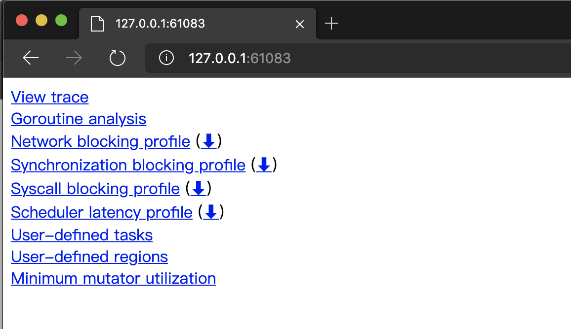
We see that the home page displays multiple hyperlinks to data analysis, each of which will open an analysis view where.
- View trace: rendering and displaying the tracer data in the form of a graphical page (see Figure 3 above), which is the feature we are most concerned about/use most often.
- Goroutine analysis: records the various trace data of multiple goroutines executing the same function in the form of a table. The table in Figure 5 below records the various data of the eight goroutines executing the same main.createColWorkers.func1.
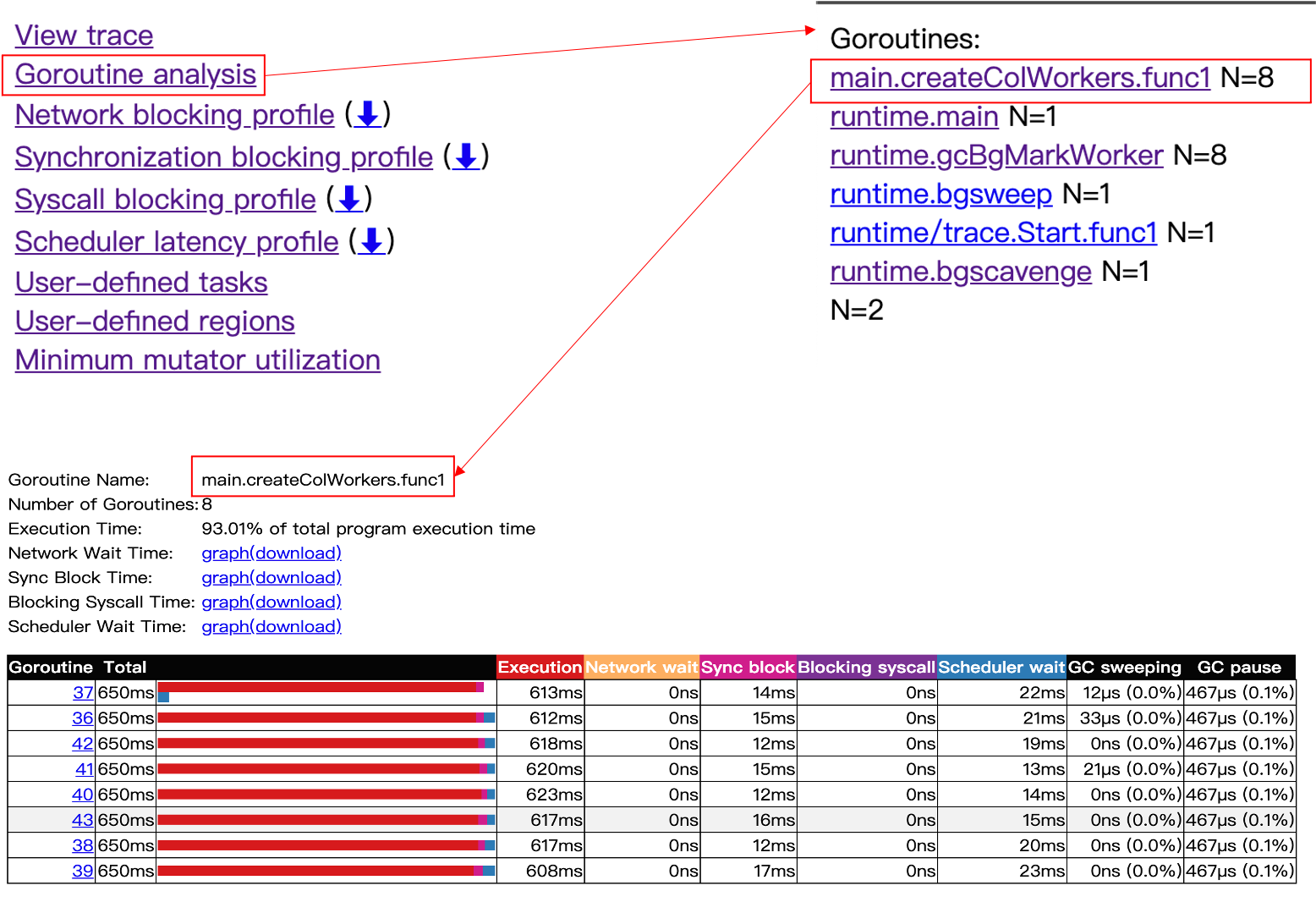
- Network blocking profile: A call relationship diagram in the form of a pprof profile showing the network I/O blocking situation
- Synchronization blocking profile: A call relationship diagram in the form of a pprof profile showing synchronization blocking time consumption
- Syscall blocking profile: A call relationship diagram in the form of a pprof profile showing system call blocking time consumption
- Scheduler latency profile: A call relationship diagram in the form of a pprof profile showing scheduler latency
- User-defined tasks and User-defined regions: user-defined task and region of trace
- Minimum mutator utilization: a graph to analyze the impact of GC on application latency and throughput
Usually we are most concerned about View trace and Goroutine analysis, and we will talk about the usage of these two in detail below.
The official documentation on Go Execution Tracer is very scarce at the moment (https://github.com/golang/go/issues/16526), especially for go tool trace analysis of each view in the tracer data process, and what you can see on the web is mostly What you can see on the web is mostly “experience data” accumulated by third parties in the process of using go tool trace.
1) View trace
Click on “View trace” to enter the Tracer data analysis view, see Figure 6 below.
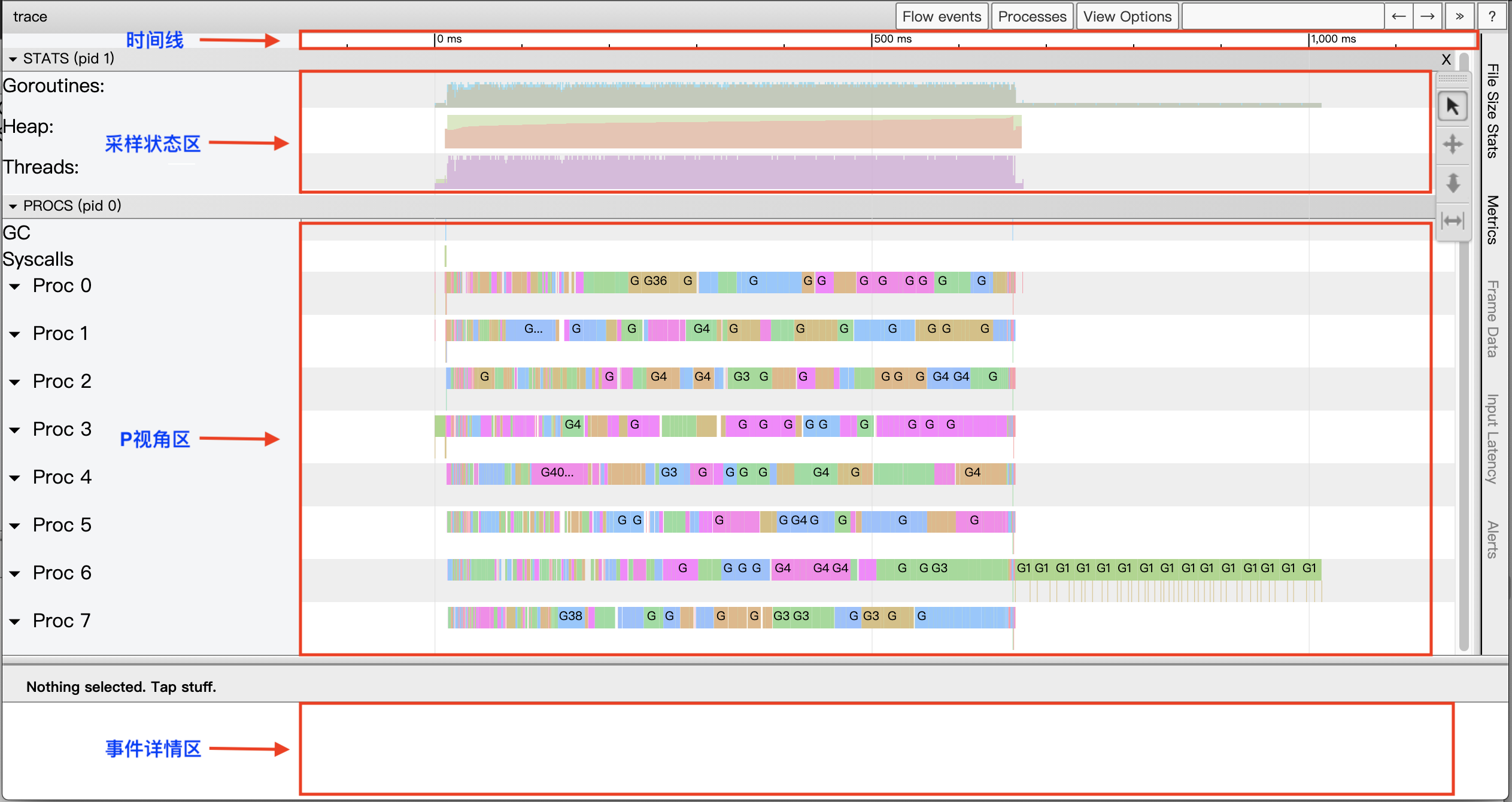
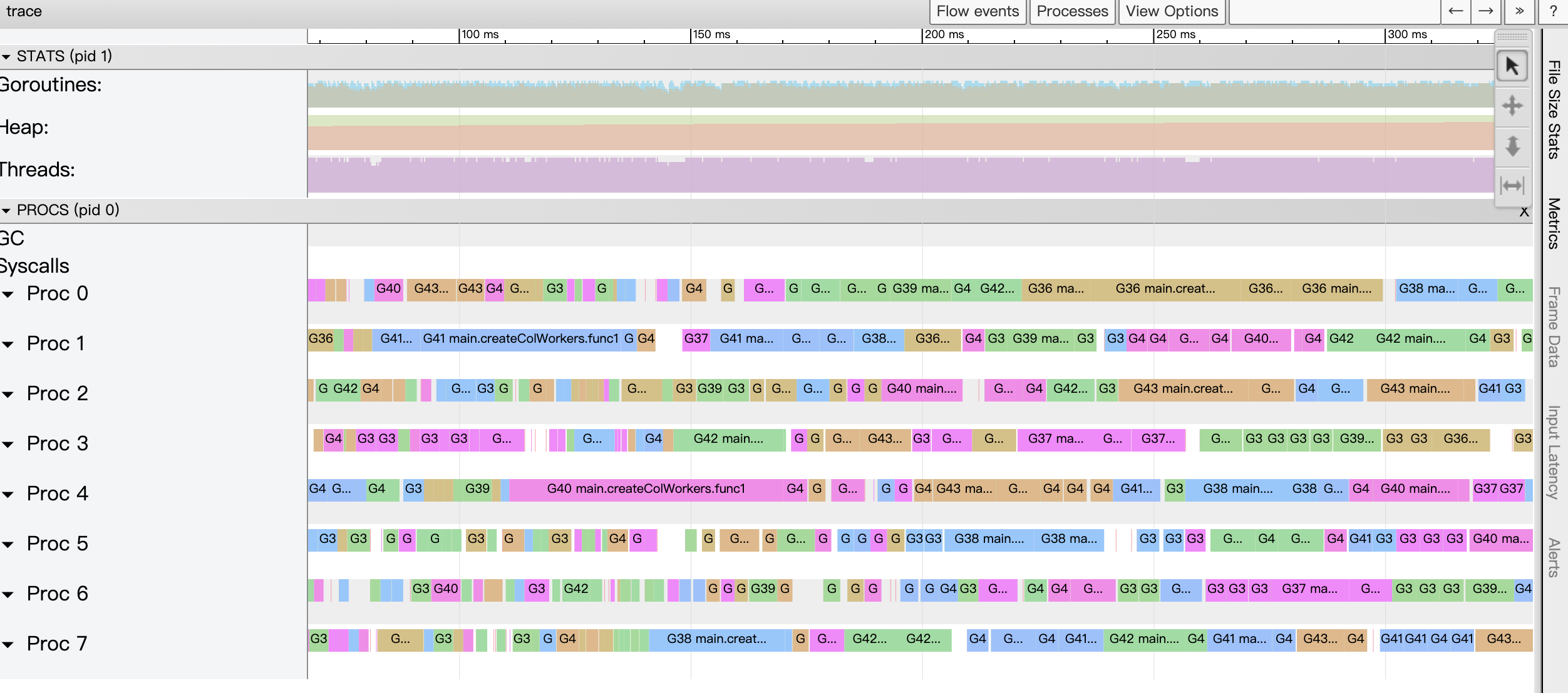
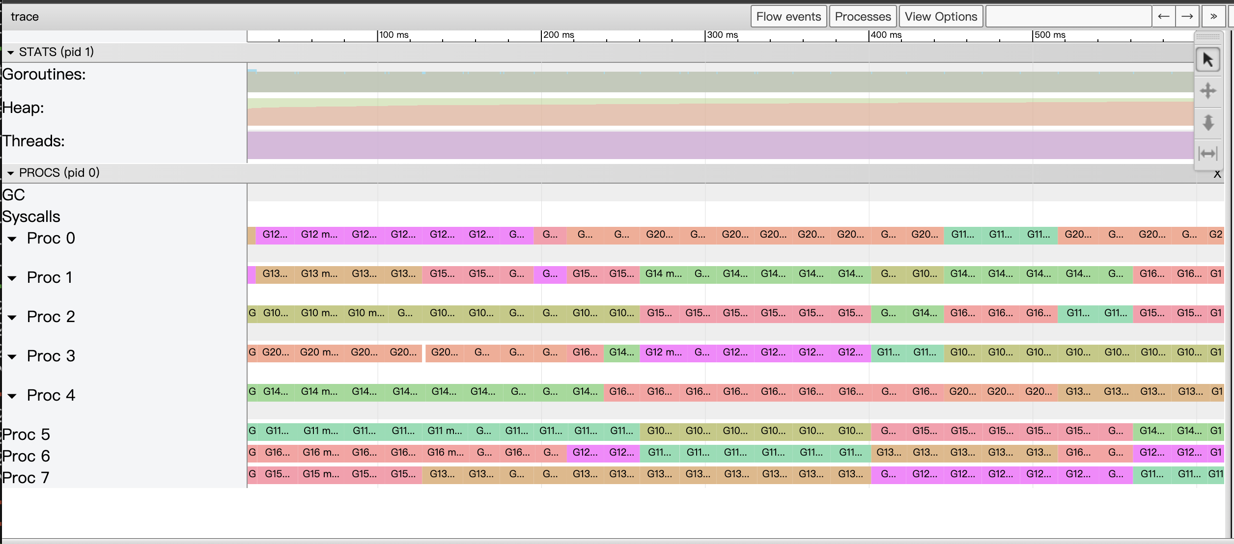
View trace view is implemented based on google’s trace-viewer, which can be roughly divided into four areas.
- Timeline (timeline)
The timeline provides a time frame of reference for the View trace. The timeline of the View trace starts when the Tracer is opened, and the time of the events recorded in each area is based on the start time of the timeline relative time .
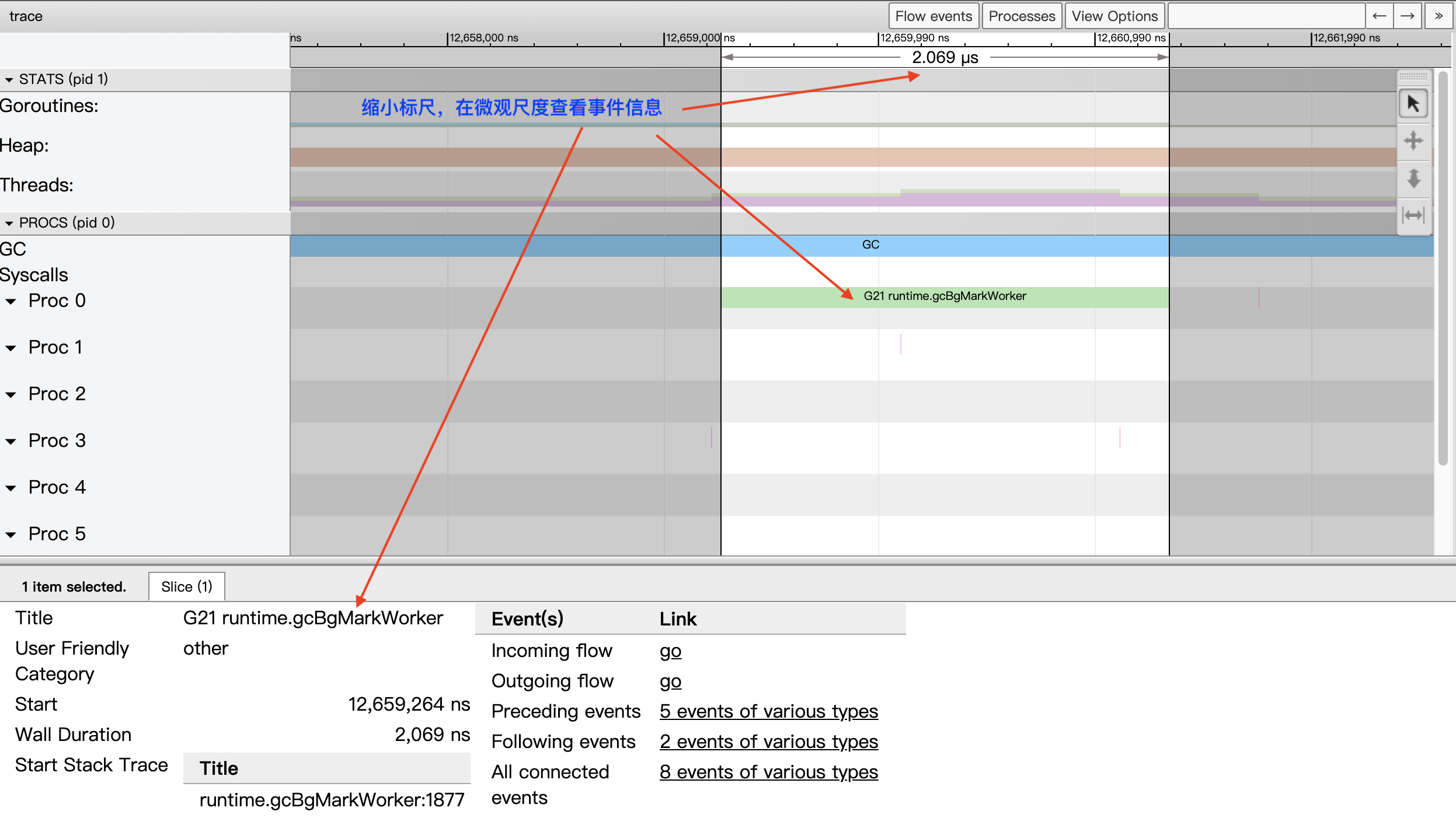
The timeline is accurate up to nanoseconds, but the View trace view supports free scaling of the timeline’s time scale, so that we can view the whole picture at the “macro scale” of seconds and milliseconds, as in Figure 6 above; we can also scale the time scale to the “micro scale” of microseconds and nanoseconds to view a particular We can also scale the time scale down to the microscopic scale of microseconds and nanoseconds to see the details of a very short event:
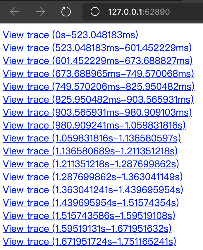
If the Tracer trace is long and the trace.out file is large, go tool trace will divide the View trace by time period to avoid hitting the limits of the trace-viewer.
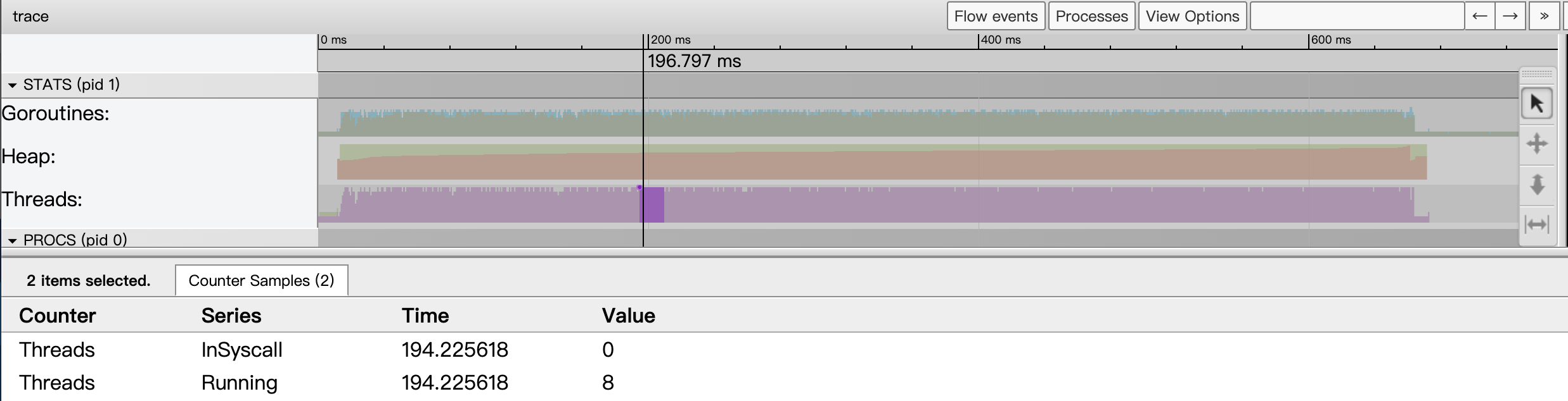
View trace uses shortcuts to scale the timeline scale: the w key for zooming in (scaling from seconds to nanoseconds) and the s key for scaling out (scaling from nanoseconds to seconds). We can also use shortcuts to move left and right on the timeline: the s key for moving left and the d key for moving right. If you can’t remember these shortcuts, you can click on the question mark in the upper right corner of the View trace view? button, the browser will bring up the View trace operation help dialog.
All shortcuts of the View trace view are available here.
- Sampling Status Area (STATS)
This area shows three metrics: Goroutines, Heap and Threads. The data for these three metrics at a point in time is a snapshot sampling of the state at that point in time.
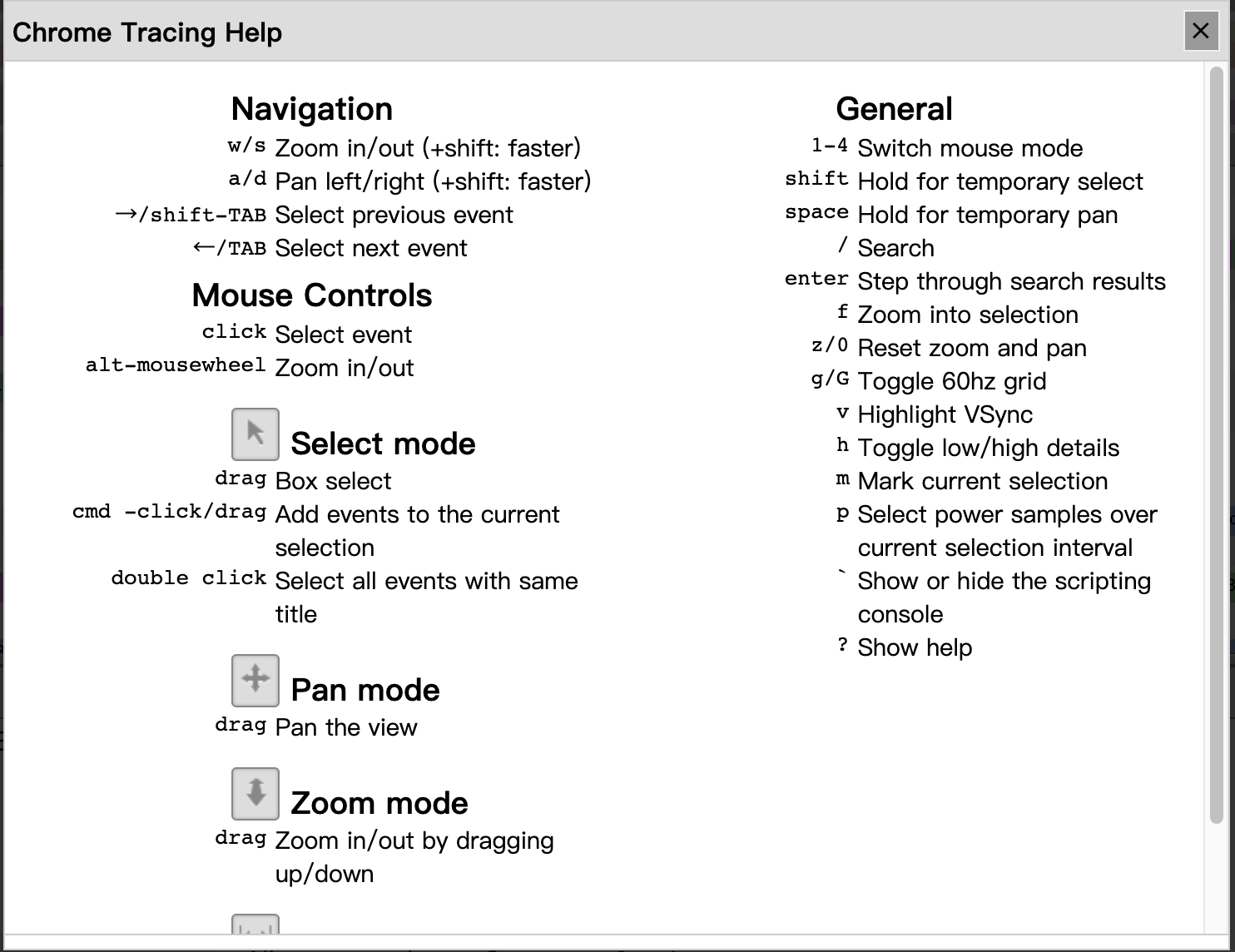
Goroutines: the number of goroutines started in the application at a certain point in time. When we click on the goroutines sampled status area at a certain point in time (we can use the shortcut m to mark exactly that point in time), the event details area will show the current goroutines indicator sampled status:
From the above figure we see that there are 9 goroutines at that point in time, 8 are running and the other 1 is ready and waiting to be scheduled. The number of goroutines in GCWaiting state is 0.
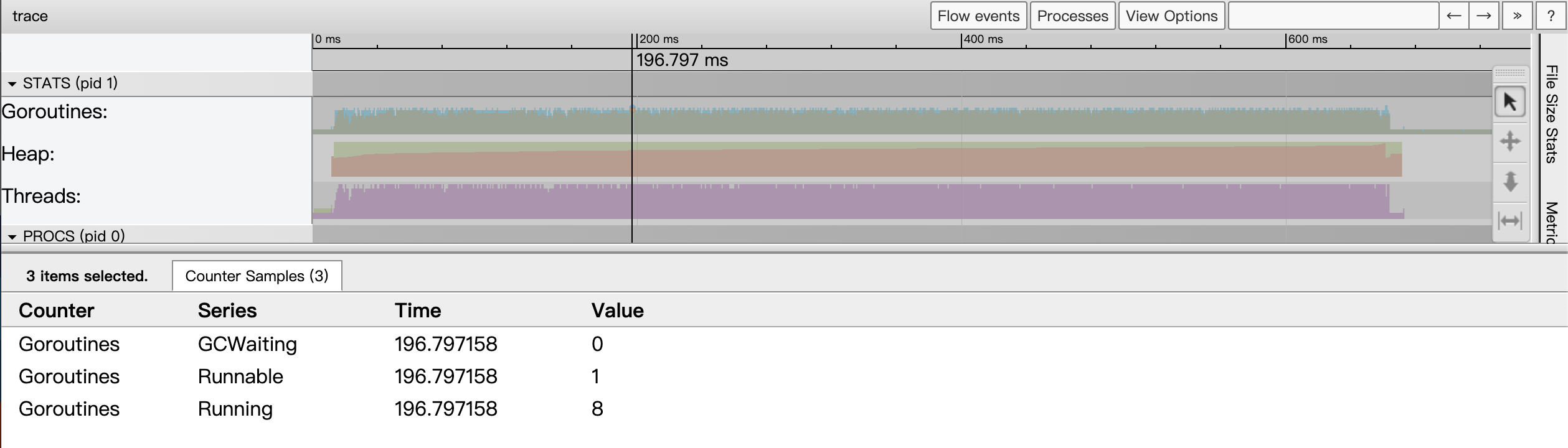
The Heap indicator, on the other hand, shows the Go application heap allocation (both Allocated and NextGC, the target value for the next GC) at a point in time.
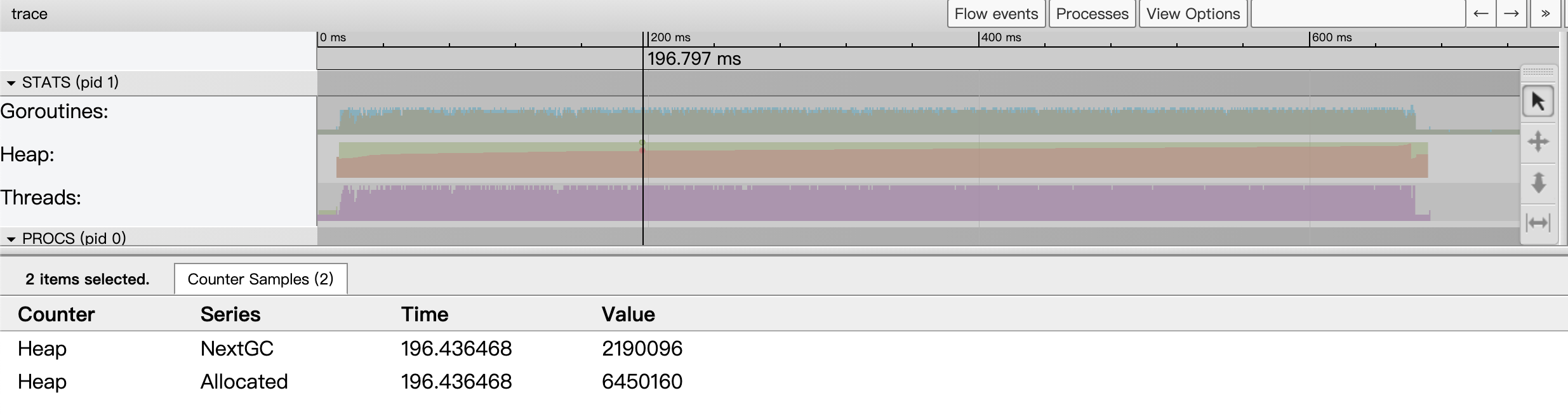
The Threads metric shows the number of threads started by the Go application at a given point in time, and the event details area will show the number of threads in both the InSyscall (blocking on a system call) and Running states.
The continuous sampling data arranged on a time line depicts the trend situation of each indicator.
- P-view area (PROCS)
The largest area of the View trace view is called the “P-view area”. This is because in this area, we can see all the events that occurred on each P (P in the Goroutine scheduling concept) in the Go application, including: EventProcStart, EventProcStop, EventGoStart, EventGoStop, EventGoPreempt, and EventGoPreempt. Goroutine assisted GC various events as well as Goroutine’s GC blocking (STW), system call blocking, network blocking, and synchronization primitive blocking (mutex) events. In addition to the events occurring on each P, we can see all the events during GC displayed in a separate line.
Also we see that each Proc corresponds to a strip with two rows, the top row represents the main event of the Goroutine running on that P, while the second row shows some other events, such as system calls, runtime events, etc., or some tasks done by the goroutine on behalf of the runtime, such as parallel tagging on behalf of the GC. The following Figure 13 shows the strips for each Proc.
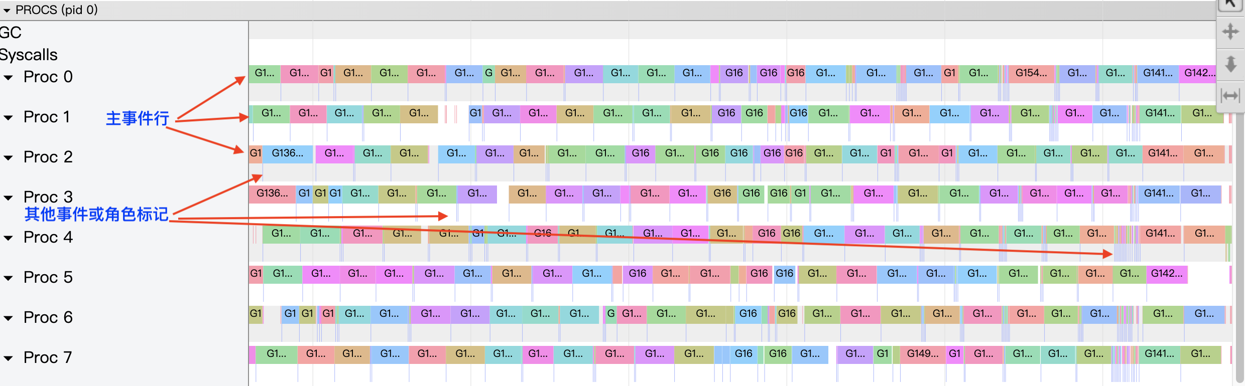
We zoomed in on the image to see the details of the stripes corresponding to Proc.
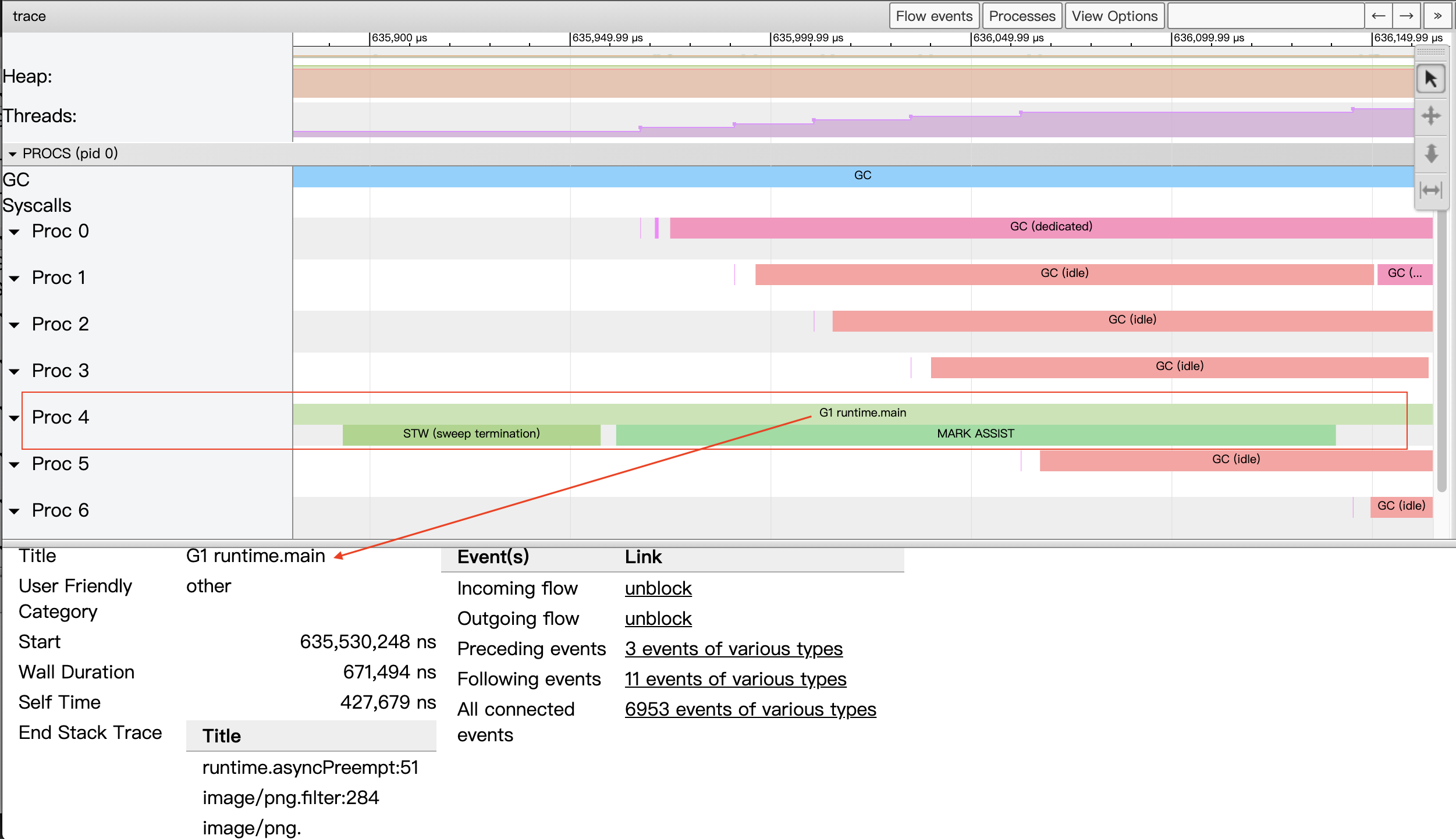
Let’s take the strip in proc4 in the figure above as an example, which contains three events. The event in the first of the two rows of the strip indicates that the goroutine G1 is scheduled to run on P4. When we select the event, we can see the details of the event in the event details area.
- Title: the readable name of the event.
- Start: the start time of the event, relative to the start time on the timeline.
- Wall Duration: the duration of this event, here the duration of this execution of G1 on P4.
- Start Stack Trace: the call stack of G1 when P4 starts the execution of G1.
- End Stack Trace: the call stack of G1 when P4 ends the execution of G1; judging from the function at the top of the End Stack Trace stack as runtime.asyncPreempt above, the Goroutine G1 is forcibly preempted so that P4 ends its operation.
- Incoming flow: the event that triggers the execution of G1 by P4.
- Outgoing flow: events that trigger the end of the execution of G1 on P4.
- Preceding events: all previous events associated with the goroutine G1.
- Follwing events: all the events after the goroutine associated with G1
- All connected: all events related to the goroutine G1.
The second line of the proc4 strip has two events occurring sequentially, one is stw, which means that GC suspends the execution of all goroutines; the other is a concurrent marker that allows G1, a goroutine, to assist in the execution of the GC process (probably because G1 allocates memory more and faster and GC chooses to let it surrender some of its arithmetic power to do the gc marker).
With the above description, we can see that with the P perspective area we can visualize the entire program (each Proc) in its entirety on the timeline of program execution, and in particular, details of the events associated with each goroutine (each goroutine has a unique separate color) running on each P in timeline order.
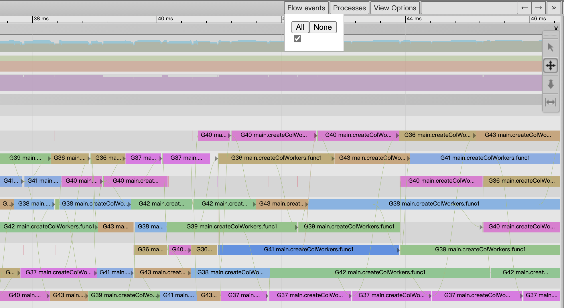
The P-view area is explicitly related to each event, and we can open the flow of related events via the “flow events” button at the top of the view, so that we can see the relationship between the events before and after an event in the diagram (Figure 15 below).
- Event details area
At the bottom of the View trace view is the Event Details area, where detailed information about an event is displayed when we click on it, as in Figure 14 above.
On a macro scale, the events in the second row of each P-band are mostly presented as a vertical line due to the short duration of the event, so it is not very easy to tap on these events. These events can be selected by either zooming in on the image or by sequentially selecting them with the two keyboard keys, left or right arrow, and then explicitly marking the event with the m key (and unmarking it by hitting the m key again).
2) Goroutine analysis
Like the sub-pages of Goroutine analysis shown in Figure 5, Goroutine analysis provides us with a G-view of the Go application execution.
By clicking on any of the Goroutine ids located in the first column of the table in Figure 5, we are taken to the Go perspective view of.
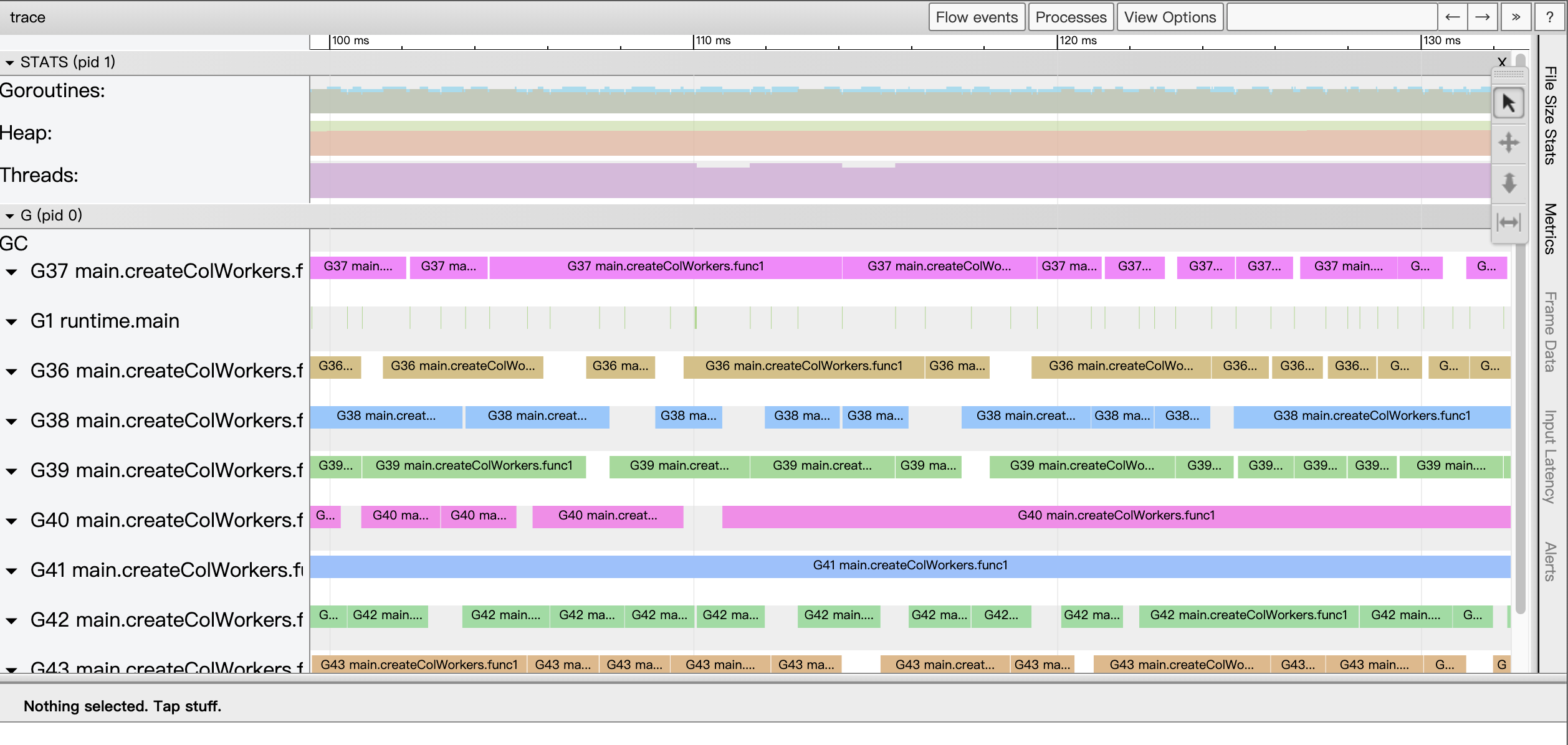
We see that unlike View trace, this time the most expansive area of the page provides a G-view view instead of a P-view view. In this view, each G corresponds to a separate strip (like the P-view, each strip has two rows), and through this strip we can see the full execution of the G by timeline. Usually we just find the two fastest and slowest executing goroutines in the table page of goroutine analysis and compare them along the timeline in the Go view to try to find out what is wrong with the slow goroutine.
4. Example Understanding
Here is an example to understand how Go Execution Tracer helps us solve a problem. It is not easy to write such an example, as Francesc Campoy has previously given in his justforfunc column a nice example that can be used for Tracer), which I borrow here ^_^.
Francesc Campoy gives an example of generating a fractal image, the first version of the code is as follows.
|
|
This version of the code uses the pixel function to calculate the value of each pixel in the image to be output, this version of the code even without pprof can basically locate the program hotspots on the pixel function on the critical path, the more accurate location is the loop in the pixel. So how to optimize it? pprof has run out of tricks, we use Tracer to see.
The view of the View trace displayed by the go tool trace is as follows.
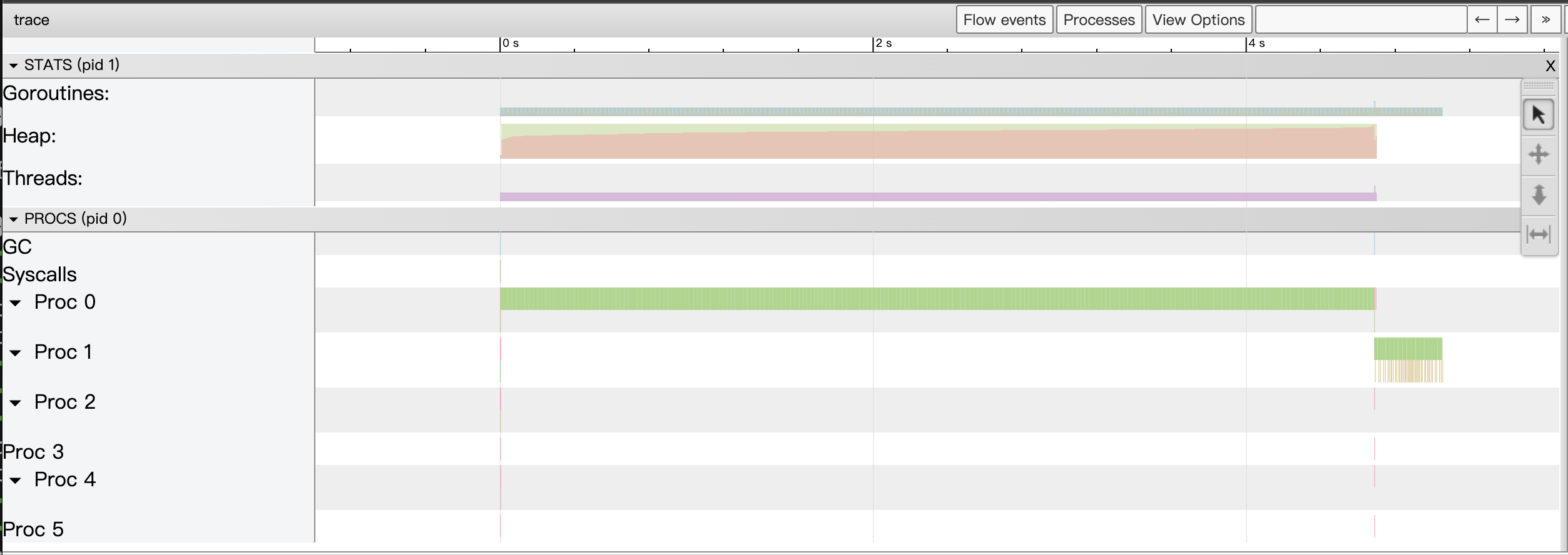
From the View trace view above, we can see at a glance that this version of the program only uses one of the multiple cpu cores on the machine, while the rest of the cpu cores are idle.
The author then gives an extreme concurrency solution, where each pixel computation starts a new goroutine (replacing createSeq in main.go with createPixcel above).
|
|
This version of the program does have improved execution performance and makes full use of the cpu, check its Tracer data (due to the large Tracer data file pixel.trace in this version, it takes a while to wait) as follows.
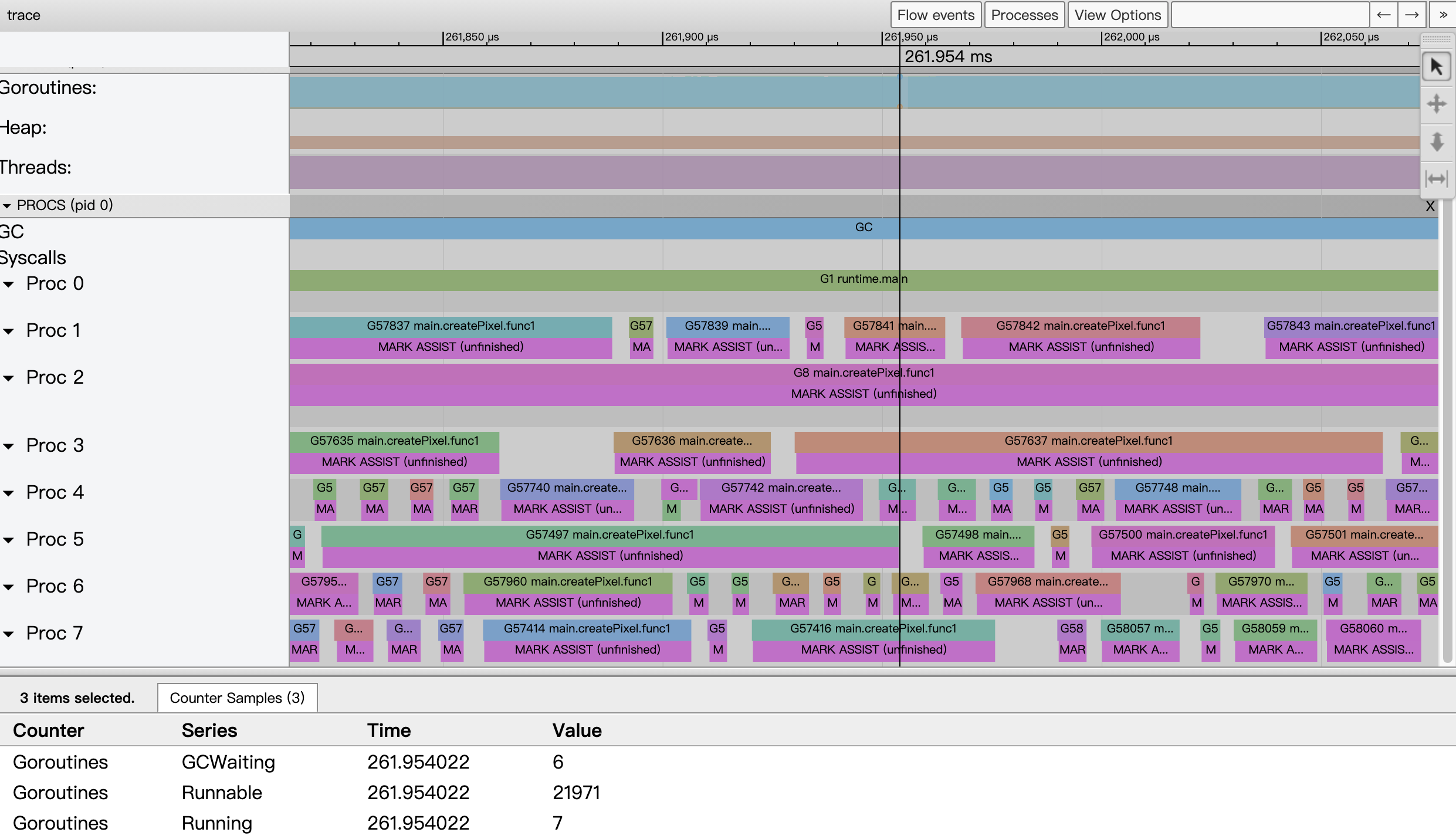
Taking the event data around 261.954ms as an example, we see that all 8 cpu cores of the system are running at full capacity, but from the state collection data of goroutines, we see that only 7 goroutines are running, while 21971 goroutines are waiting to be scheduled, which puts a lot of pressure on the scheduling of go runtime; in addition, since This version of the code creates 2048×2048 goroutines (more than 400w), which leads to frequent memory allocation and puts a lot of pressure on the GC, and from the view, each goroutine seems to be assisting the GC in parallel marking. This shows that we cannot create so many goroutines, so the author gives a third version of the code, creating only 2048 goroutines, each goroutine being responsible for the generation of one column of pixels (replacing createPixel with the following createCol).
|
|
This version of the code works like a charm! Almost 5 times better performance. Can it be further optimized? So the authors implemented another version of the code based on the Worker concurrency pattern.
|
|
The author’s machine is an 8-core host, so it pre-created 8 worker goroutines, with the main goroutine dispatching work to each goroutine via a channel c. However, the author did not see the expected performance, which was not as good as the version with one goroutine per pixel. Check the Tracer situation as follows (this version of the code has more Tracer data and takes longer to parse and load).
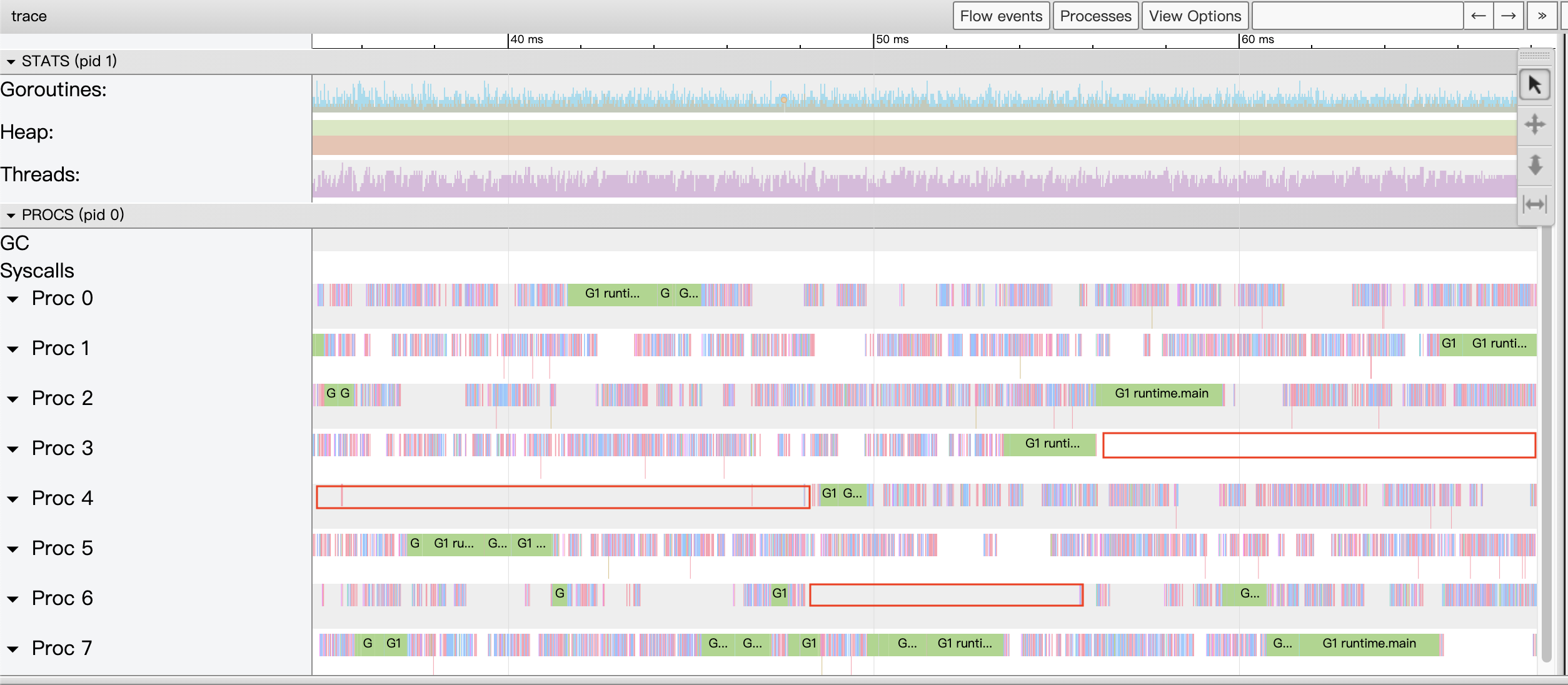
We see a properly zoomed in View trace view, we see a lot of large Proc pauses and countless small pauses, obviously the goroutine is blocking, we then go through the Synchronization blocking profile to see exactly where the blocking time is the longest.
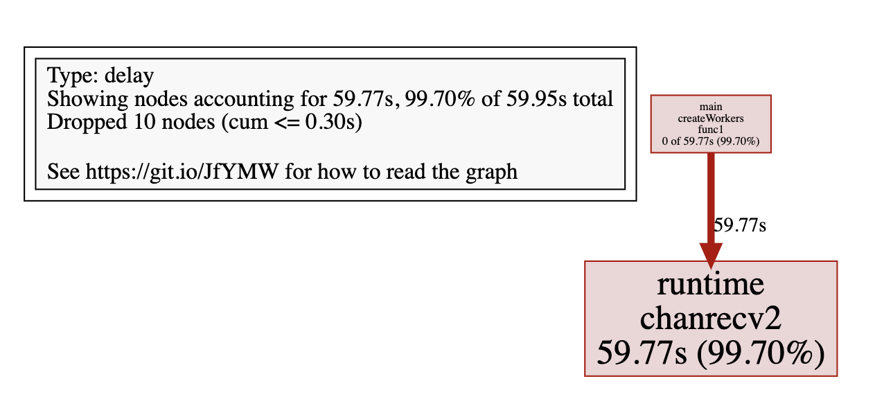
We see that all goroutines wait for nearly 60s on channel reception. From this version of the code, the main goroutine has to send more than 400 times, while the other 8 worker goroutines have to wait patiently on the channel reception, which is obviously not an optimal structure.
The authors came up with the idea of createCol, i.e. instead of sending each pixel as a task to a worker, a column is sent to a worker as a work unit, and each worker completes the computation of a column of pixels, which brings us to the final version of the code (using the following createColWorkersBuffered replacement createWorkers).
|
|
This version of the code does have the best performance of all versions, with the following View trace view of the Tracer.
This is almost a perfect View trace view!
5. Summary
Go Execution Tracer is not a silver bullet, it can’t help you solve all the problems in your Go application. Usually when doing performance analysis on Go applications, we use pprof to find hotspots first, and then after eliminating them, we use Go Execution Tracer to look at the execution of goroutines in the whole Go application in a holistic way, find out the problematic points through View trace or Goroutine analysis and analyze them in detail.
Parallelism, latency, goroutine blocking and other aspects of Go applications are the “main battlefield” that Go Execution Tracer is good at.