Operating system process scheduling algorithm

This article summarizes the process scheduling algorithms of the operating system and analyzes the advantages and disadvantages, including the FIFO algorithm, the shortest task priority algorithm, the rotation algorithm, the multi-level feedback queue algorithm, the lottery scheduling algorithm, and the multi-processor scheduling algorithm. Only the principles of each algorithm are summarized, but not the specific implementation of Linux scheduling algorithms.

Scheduling Metrics

Before looking at the process scheduling algorithm, let’s see what metrics are followed by the process scheduling algorithm. For now, only turnaround time and response time are considered.

Turnaround time: the time for a task to complete minus the time for the task to arrive at the system. Response time: the time from when the task arrives at the system to when it first runs.

Performance and fairness are often contradictory in scheduling systems; for example, schedulers can optimize performance at the cost of preventing some tasks from running, which reduces fairness.

FIFO

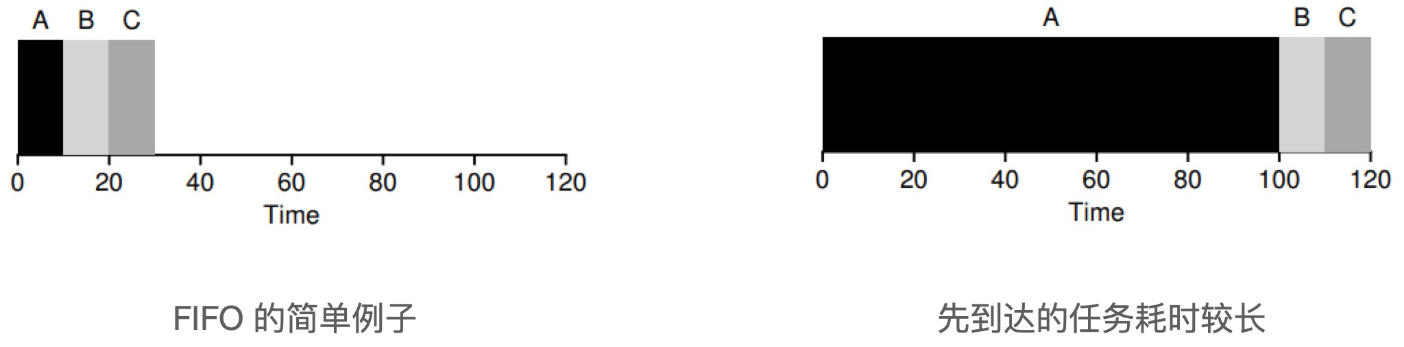
FIFO is First In First Out (FIFO), sometimes also called First Come First Served (FCFS).

• Pros: Very simple and easy to implement.
• Disadvantage: The average turnaround time of the FIFO scheduling algorithm can be very long when the task that arrives first takes a long time.

Shortest Job First (SJF)

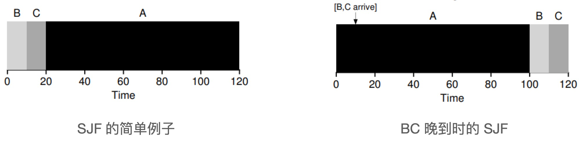
The strategy of the Shortest Job First (SJF) algorithm is to run the shortest task first, then the next shortest task, and so on.

Under the assumption that all tasks arrive at the same time, SJF is indeed the optimal scheduling algorithm. However, SJF is not optimal when there are first and second tasks, as shown in the figure below.

Shortest Time-to-Completion First (STCF)

The Shortest Time-to-Completion First (STFT) algorithm was introduced to solve the SJF problem, provided that the operating system allows task preemption.

STCF algorithm adds preemption to SJF, also known as Preemptive Shortest Job First (PSJF). Whenever a new job enters the system, it determines which of the remaining jobs and the new job has the least amount of time left, and then schedules the job.

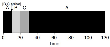
STCF is a good strategy when the task length is known and the task uses only the CPU and the only metric is the turnaround time. But considering the response time, the STCF algorithm performs quite badly, for example if you type in front of a terminal and have to wait 10s to see a response from the system, just because some other job has been scheduled before that.

Rotation Algorithm

To solve the problem of long response times of the STCF algorithm, Rotation Scheduling (Round-Robin, RR) was introduced.

The idea of Round-Robin scheduling: RR runs a job within a time slice (sometimes called a scheduling quantum) and then switches to the next job in the run queue, instead of running a job until it finishes. rR is sometimes called a time slice, and the length of the time slice must be a multiple of the clock interrupt period.

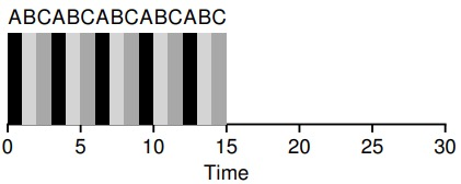
Time slice length is critical to RR. The shorter the time slice, the better the RR will perform in terms of response time. However, time slices that are too short are problematic: the cost of abrupt context switching will affect overall performance. Therefore, system designers need to weigh the length of the time slice to make it long enough to amortize the cost of context switching without making the system unresponsive.

Note: The cost of context switching comes from more than just the OS operations of saving and restoring a small number of registers. As programs run, they build up a large amount of state in the CPU cache, TLB, branch predictors, and other on-chip hardware. Switching to another job causes this state to be refreshed and new state associated with the currently running job to be introduced, potentially resulting in significant performance costs.

Combined I/O

When a running program is performing an I/O operation, the CPU is not used during the I/O, but it is blocked waiting for the I/O to complete, at which point the scheduler should schedule another job on the CPU.

Instead, when the I/O completes, an interrupt is generated and the OS runs and moves the process that issued the I/O from the blocking state back to the ready state. Of course, it can even decide to run the job at that time. How should the OS handle each job?

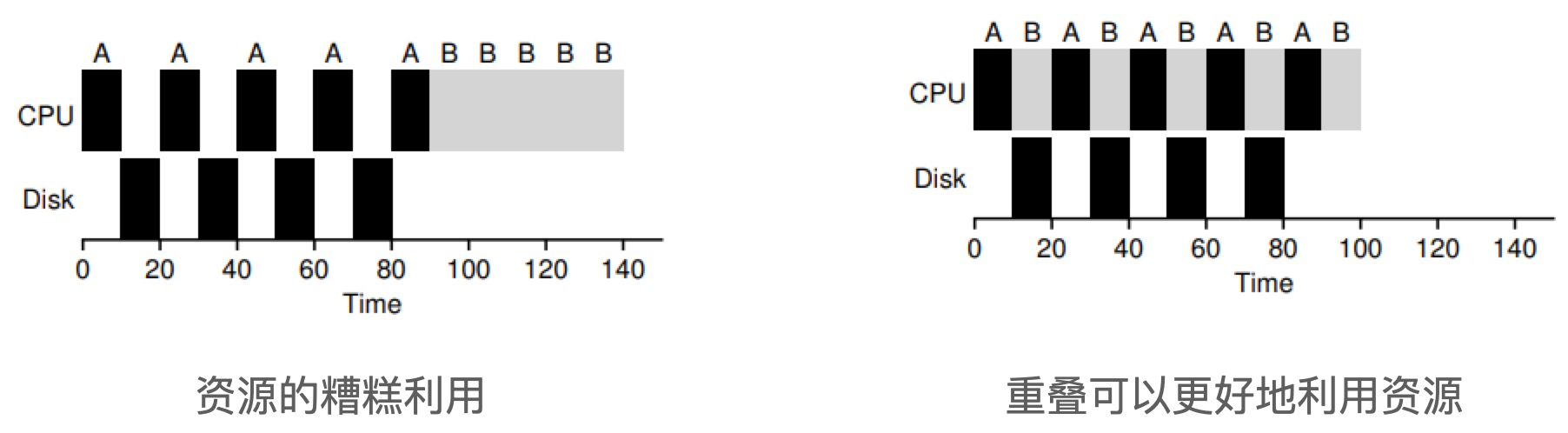
Suppose there are two jobs A and B, each requiring 50ms of CPU time. But A runs 10ms first, then issues I/O requests (assuming I/O takes 10ms each), while B just uses the CPU for 50ms and does not perform I/O. The scheduler runs A first, then B.

The scheduling shown on the left is very bad. A common approach is to treat each 10ms subjob of A as a separate job. Thus, when the system starts, its choice is whether to schedule 10ms of A or 50ms of B. STCF will choose the shorter A. Then, the work of A is completed, leaving only B, and it starts running. Then a new subjob of A is submitted, which grabs B and runs for 10ms. this allows for overlap, one process uses the CPU while waiting for another process’ I/O to complete, and the system is thus better utilized.

Multi-level feedback queues

The operating system often does not know how long the job will run, which is necessary for algorithms such as SJF; and while rotational scheduling reduces response time, turnaround time is poor. This led to the introduction of the Multi-level Feedback Queue (MLFQ), which needed to solve two problems: first, it needed to optimize turnaround time, which could be achieved by prioritizing the execution of shorter jobs; second, MLFQ wanted to provide a better interaction experience for the user, so it needed to reduce response time.

There are many independent queues in MLFQ, each with a different priority. At any given time, a job can exist in only one queue, and MLFQ always prioritizes the higher priority jobs (i.e., those in higher queues). There may be multiple jobs in each queue that have the same priority. In this case, we use rotational scheduling for these jobs.

Basic rules

The multilevel feedback queue consists of several basic rules.

• Rule 1 : If the priority of A is greater than the priority of B, run A without running B.
• Rule 2 : If A’s priority is equal to B’s priority, run A and B in rotation.
• Rule 3: Jobs are placed in the highest priority (top) queue when they enter the system. This rule makes the multi-level feedback queueing algorithm similar to SJF and ensures good response times.
• Rule 4 : Once a job has used up its time quota in a tier (regardless of how many times it actively abandons CPUs in between), it is lowered in priority (moved to a lower tier queue). This rule prevents processes from actively giving up CPUs and thus starving other processes.
• Rule 5 : Every time a period of time passes, all work in the system is rejoined to the highest priority queue. This rule solves two problems: one is to prevent starvation of long processes, and the other is that if a CPU-intensive job becomes interactive, the scheduler treats it correctly when it is given a higher priority.

Proportional share

The proportional-share scheduler, sometimes called the fair-share scheduler. The proportional-share algorithm assumes that the ultimate goal of the scheduler is to ensure that each job gets a certain percentage of CPU time, rather than optimizing turnaround time and response time. Its basic idea is simple: every once in a while, a lottery draw is held to determine which process should be run next. The more frequently a process should be run, the more chances it should have to win the lottery.

Lottery numbers represent shares

In lottery scheduling, the number of lotteries represents the share of a process in possession of a particular resource. The number of lotteries a process owns as a percentage of the total number of lotteries is the share of the resource it occupies.

Suppose there are two processes A and B. A owns 75 lottery tickets and B owns 25. So we want A to take 75% of the CPU time and B to take 25%.

By constantly and regularly drawing lottery tickets, lottery scheduling gets this share ratio from probability. The process of drawing tickets is simple: the scheduler knows the total number of tickets (in our case, 100). The scheduler draws the winning ticket, which is a number between 0 and 99, and the process that has the ticket corresponding to this number wins the lottery. Suppose process A has 75 tickets from 0 to 74 and process B has 25 tickets from 75 to 99. The winning ticket determines whether to run A or B. The scheduler then loads the state of the winning process and runs it. Lottery scheduling takes advantage of randomness, which results in a ratio that probabilistically meets expectations. As these two jobs run longer, the closer the ratio of CPU time they get to the expectation.

Implementation

Lottery scheduling is very simple to implement, requiring only a random number generator to select the winning tickets and a data structure to record all processes in the system, as well as the total number of all tickets. Suppose we use a list to record the processes, the following example has 3 processes A, B and C, each with a certain number of lottery tickets.

Step scheduling

Although the random approach can make the implementation of the scheduler simple, occasionally it does not produce the correct ratio, especially if the job has a short run time. For this reason, Waldspurger proposed step scheduling.

Each job in the system has its own step length, and this value is inversely proportional to the number of votes. 3 jobs, A, B, and C, have votes of 100, 50, and 250, respectively, and we obtain the step length of each process by dividing each of their votes by a large number. For example, dividing these vote values by 10,000 gives us the step lengths of the 3 processes of 100, 200 and 40. we call this value the step length (stride) of each process. After each process runs, we let its counter (called trip value) increase its stride length and record its overall progress.

The basic idea: when scheduling is needed, select the process that currently has the smallest stroke value and increase that process’s stroke value by one step after it runs.

Pseudocode.

1
2
3
4

current = remove_min(queue);       // pick client with minimum pass
schedule(current);                 // use resource for quantum
current->pass += current->stride;  // compute next pass using stride
insert(queue, current);            // put back into the queue

The advantage of lottery scheduling over step scheduling is that it does not require global state. If a new process joins the system during the execution of step scheduling, how should I set its trip value? Should it be set to 0? In that case, it would be exclusive to the CPU. The lottery scheduling algorithm, on the other hand, does not need to record the global state for each process, but only needs to update the global total number of votes with the number of votes of the new process. Thus the lottery scheduling algorithm can handle the newly added processes more reasonably.

Multiprocessor Scheduling

The above scheduling algorithms are all single-processor scheduling, while when the operating system uses multi-core CPUs, multi-processor scheduling must be considered.

Multiprocessor Architecture

The basic difference between a multiprocessor and a single CPU centers on the use of hardware cache and the way data is shared between multiprocessors.

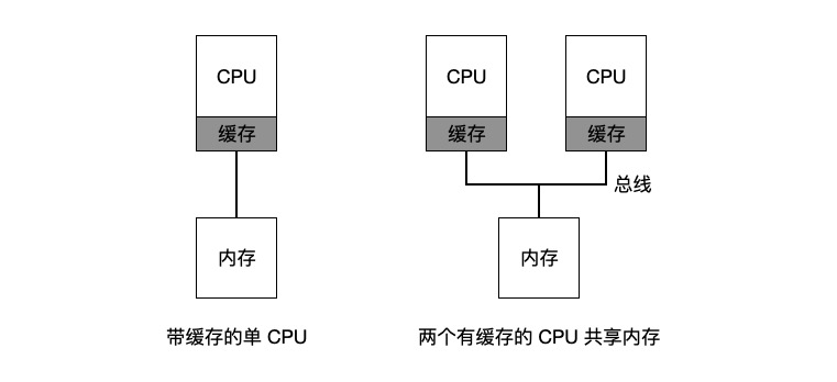
In a single CPU system, the presence of all the hardware cache that is available will generally allow the processor to execute programs faster. Caches are small but fast storage devices that typically hold a backup of the hottest data in memory. In contrast, memory is large and holds all the data, but is very slow to access. By putting frequently accessed data in the cache, the system appears to have a large and fast memory.

And when there are multiple CPUs, there is a cache coherency problem. Hardware provides the basic solution to this problem: by monitoring memory accesses, hardware can ensure that the correct data is obtained and that the shared memory is unique.

There is one more issue to consider with multiprocessor scheduling: cache affinity. A process running on a CPU maintains many states in that CPU’s cache, so multiprocessor scheduling should take this cache affinity into account and keep the processes on the same CPU as much as possible.

Single Queue Scheduling

The most basic way to schedule a multiprocessor system is to simply reuse the basic architecture of single-processor scheduling and put all the jobs to be scheduled into a single queue, which is called Single Queue Multiprocessor Scheduling (SQMS).

Shortcomings of SQMS:

1. Lack of scalability. To ensure proper operation on multiple CPUs, the scheduler needs to ensure atomicity in the code by adding locks, which can result in significant performance loss.

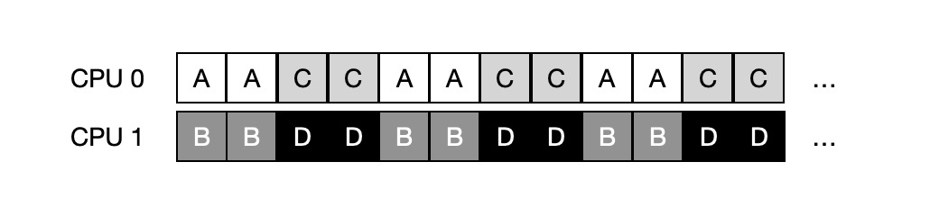
2. cache affinity issues. For example, if there are 5 jobs A, B, C, D, E and 4 processors in the queue, and after a period of time it is assumed that each job executes one time slice at a time and then another job is selected, the following is the possible scheduling sequence of CPUs.

   

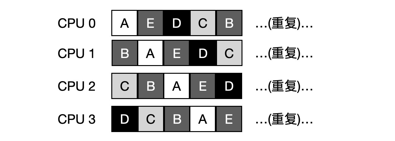
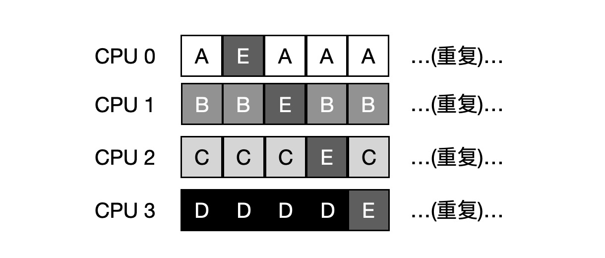
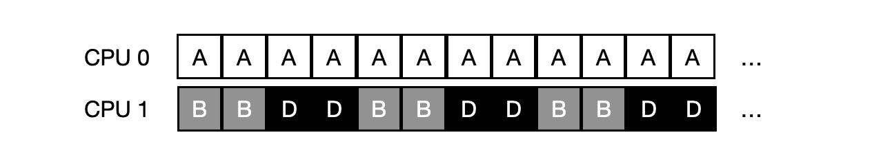
To solve this problem, most SQMS schedulers introduce some affinity mechanism to keep the incoming jobs running on the same CPU as much as possible. For example, the scheduling for the same 5 jobs is as follows, with 4 jobs A, B, C, and D staying on the same CPU and only E constantly migrating back and forth.

Multi-queue Scheduling

It is due to these problems with single-queue scheduling that some systems use a multi-queue scheme, such as one queue per CPU, which we call Multi-Queueue Multiprocessor Scheduling (MQMS).

In MQMS, the basic scheduling framework contains multiple scheduling queues, each of which can use different scheduling rules. When a job enters the system, it is placed in a scheduling queue according to some initiation rules. Each CPU scheduling is independent of each other, thus avoiding the problems associated with data sharing and synchronization in a single-queue approach.

For example, suppose there are two CPUs in the system and jobs A, B, C, and D enter the system, each CPU has its own scheduling queue, and the OS feels which queue to put each job into, e.g.

Depending on the scheduling policy for the different queues, each CPU chooses from two jobs to decide who will run, e.g. using rotation, and the scheduling result may look like the following.

But this is bound to have the problem of uneven load.

Let’s say job C finishes executing at this point, and the scheduling queue is now as follows.

And the rotation scheduling results are as follows.

To make matters worse, if A and C both finish executing and the system only has B and D, the scheduling queue looks like this.

So the CPU timeline looks sad:

At this point, the solution to this load imbalance is migration. By working with cross-CPU migration, load balancing can be truly achieved.

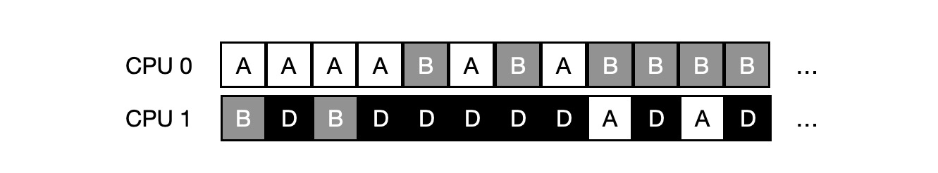
In the example above, load balancing is achieved by migrating B or D to CPU 0. In the earlier example, however, A is left alone on CPU 0, while B and D are running alternately on CPU 1. In this case, a single migration does not solve the problem and one or more jobs should be migrated continuously. One possible solution is to keep switching jobs, as shown in the timeline below. As you can see, at the beginning, A has exclusive access to CPU 0, B and D are on CPU 1, and after a period of slices, B migrates to CPU 0 and competes with A, while D has exclusive access to CPU 1 for a period of time. This achieves load balancing.

One of the most basic ways to implement task migration is work stealing (work stealing). In this method, a queue with less work is “stealing” from other queues from time to time to see if they have more work than they do. If the target queue is fuller than the source queue, one or more jobs are “stolen” from the target queue to achieve load balancing.

Linux Multiprocessor Scheduling

There has been no consensus in the Linux community on building a multi-processor scheduler. There have been three different schedulers: the O(1) scheduler, the Completely Fair Scheduler (CFS), and the BF scheduler (BFS).

O(1) and CFS use multiple queues, while BFS uses a single queue; O(1) scheduler is priority-based (similar to MLFQ), changing the priority of processes over time and then scheduling the highest priority processes to achieve various scheduling goals; CFS is a deterministic proportional scheduling method (similar to step scheduling); BFS is also proportional-based scheduling, but uses a more sophisticated precaution called the Earliest and Best Fit Virtual Deadline First algorithm (EEVEF).